Application of XGBoost regression for Spatial Interaction of Urban flow
Gravity based model with Gradient Boosting Trees
Introduction
This notebook provides a simple example of the application of XGBoost Spatial Interaction model in python. For the purposes of this tutorial I will expect you to have some knowledge of Spatial Interaction Models and their purpose as well as some python skills. Yet, if you want to refresh a little or wish to learn, here is a list of relevant sources.
- Watch Maarten Vanhoof talking about what are the spatial Interaction Models and how they can be used here (6 min)
- Have a look at a list of some relevant literature in different fields here
- Look at the example of Spatial Interaction Model application in R from Adam Dennett Part1 and Part2
- Look at how you can apply the the same method in python with SpInt package
So what is the XGBoost? and how does it work?
XGBoost stands for “Extreme Gradient Boosting”, where the term “Gradient Boosting” originates from the paper Greedy Function Approximation: A Gradient Boosting Machine, by Friedman. Please have a look at this A Gentle Introduction to XGBoost for Applied Machine Learning and the Full documentation to XGBoost that also provides a tutorials. If you are like me and need something more visual and efficient explanation of the how the model works, I would highly recommend YouTube videos from Josh Starmer; Gradient Boost Part 1: Regression Main Ideas, Gradient Boost Part 2: Regression Details.
So after you gone through all the resources you know that there are two types of the model depending on what do you want to do with them. You can use them as a classifier, similar to decision trees, or as a regressor. Using the method as a classifier, we can predict discrete and categorical variables, and using it as a regressors, continuous variables can be predicted. Here we will be talking solely about Gradient Boosting as a regressor, because we are trying to model Urban flow, number of people that moves from one point to another.
What is an Urban flow here?
In this example, I am looking at patients Urban flow. to be specific, this is a patients that are being treated at particular GP, receive a prescription and then go to one of the pharmacies to pick up the prescribed drug. This process of prescribing and dispensing a drug is closely monitored by the National Health Service, although the precise information about the patients is disclosed, the NHS Digital provides completely anonymised data of number of the prescriptions that has been prescribed and dispensed between each pair of GP and Pharmacy each month. Those can be translated as traces of patients movement between two points and together creates rich network of patients flow.
For further description of the data follow up on this notebook.

Cross validation challenge
With any ordinary data, we would usually divide the data into testing set and training set by 80/20 split or any other proportion. However, we face more difficult case here.
The Urban flow networks are very particular case of network, which is basically a representation of the human behaviour in a space. And this is related to anything that affect our decision to choose a destination and the journey to it. Starting from maps, road or public transport structure and the type of vehicle, ending with our personal preference, gender, or family status. The network that the humans created by acting in it has very complex pattern in which the existence of a destination and its location matters.
Now, imagine we would divide the dataset into training and testing, how do we decide which locations will be for training and which ones will be for testing if each location is unique? For example, if we train the model on the flow data in a Scotland, we cannot test the same model on the data from London as people in both places has different behavioural patterns. There is more to it, read through this study that provides nice overview.
Luckily, the data I collected ranges from 2013 to mid-2019, which means that we can divide the data into blocks with the same timeframe. In this case I will use the data from 2017 for training and data from 2018 for testing. This block cross validation is only possible thanks to the consistent data.
Let's get started
Load the libraries
import xgboost as xgb # xgboost model library
import numpy as np # array manipulation
import pandas as pd # dataframe manipulation library
import geopandas as gpd # spatial data frame manipulatioon library
import statsmodels.api as sm
from sklearn.model_selection import train_test_split  # take out the validation packages from scikit.learn
from sklearn.model_selection import GridSearchCV
from sklearn.metrics import mean_squared_error
import matplotlib.pyplot as plt # plotting
import seaborn as sns
Load the 2017 train data
# define the path
file = r'./../.././data/NHS/working/year_data_flow/predicted_flow_2017.csv'
# read the flow file
fl17 = pd.read_csv(file, index_col=None)
# define the path
file = r'./../.././data/NHS/working/year_data_flow/complete_predicted_flow_2017.csv'
# read the flow file
cfl17 = pd.read_csv(file, index_col=None)
fl17.head()
| P_Code | P_Name_x | P_Postcode | D_Code_x | D_Name_x | D_Postcode | N_Items | N_EPSItems | Date | loop | ... | P_full_address_y | P_Status_Code_y | P_Sub_type_y | P_Setting_y | P_X_y | P_Y_y | CODE | POSTCODE | NUMBER_OF_PATIENTS | yhat | |
|---|---|---|---|---|---|---|---|---|---|---|---|---|---|---|---|---|---|---|---|---|---|
| 0 | L81004 | PORTISHEAD MEDICAL GROUP | BS20 6AQ | FA251 | HORIZON PHARMACY LTD | BS34 6AS | 130.0 | 0.0 | 2017-01-01 | False | ... | PORTISHEAD MEDICAL GROUP,PORTISHEAD MEDICAL GR... | A | B | 4 | -2.767318 | 51.482805 | L81004 | BS20 6AQ | 18363 | 0.044989 |
| 1 | L81004 | PORTISHEAD MEDICAL GROUP | BS20 6AQ | FA613 | DOWNHAM FB LTD | BS7 9JT | 39.0 | 0.0 | 2017-01-01 | False | ... | PORTISHEAD MEDICAL GROUP,PORTISHEAD MEDICAL GR... | A | B | 4 | -2.767318 | 51.482805 | L81004 | BS20 6AQ | 18363 | 0.240777 |
| 2 | L81004 | PORTISHEAD MEDICAL GROUP | BS20 6AQ | FCL91 | MYGLOBE LTD | BS15 4ND | 12.0 | 0.0 | 2017-01-01 | False | ... | PORTISHEAD MEDICAL GROUP,PORTISHEAD MEDICAL GR... | A | B | 4 | -2.767318 | 51.482805 | L81004 | BS20 6AQ | 18363 | 0.001761 |
| 3 | L81004 | PORTISHEAD MEDICAL GROUP | BS20 6AQ | FCT35 | LLOYDS PHARMACY LTD | BS20 7QA | 661.0 | 0.0 | 2017-01-01 | False | ... | PORTISHEAD MEDICAL GROUP,PORTISHEAD MEDICAL GR... | A | B | 4 | -2.767318 | 51.482805 | L81004 | BS20 6AQ | 18363 | 2393.873899 |
| 4 | L81004 | PORTISHEAD MEDICAL GROUP | BS20 6AQ | FDD77 | JOHN WARE LIMITED | BS20 6LT | 4058.0 | 0.0 | 2017-01-01 | False | ... | PORTISHEAD MEDICAL GROUP,PORTISHEAD MEDICAL GR... | A | B | 4 | -2.767318 | 51.482805 | L81004 | BS20 6AQ | 18363 | 2149.320471 |
5 rows × 77 columns
Load the 2018 test data
# first get the 018 data in, those will be the test data
file = r'./../.././data/NHS/working/year_data_flow/predicted_flow_2018.csv'
# read the flow file
fl18 = pd.read_csv(file, index_col=None)
# define the path
file = r'./../.././data/NHS/working/year_data_flow/complete_predicted_flow_2018.csv'
# read the flow file
cfl18 = pd.read_csv(file, index_col=None)
cfl18.head()
| P_Code | D_Code_new | Date | Density | NUMBER_OF_PATIENTS | N_Items | Euc_distance | great_circle_dist | predicted | |
|---|---|---|---|---|---|---|---|---|---|
| 0 | L81004 | FA696 | 2018-01-01 | 36.696000 | 18615 | 8.0 | 0.224446 | 16.560437 | 0.000777 |
| 1 | L81004 | FCT35 | 2018-01-01 | 34.918367 | 18615 | 21.0 | 0.009198 | 0.653229 | 1963.680982 |
| 2 | L81004 | FDD77 | 2018-01-01 | 29.092308 | 18615 | 5309.0 | 0.014101 | 0.983999 | 1673.379704 |
| 3 | L81004 | FD125 | 2018-01-01 | 28.670000 | 18615 | 26.0 | 0.177172 | 12.816035 | 0.030142 |
| 4 | L81004 | FEA59 | 2018-01-01 | 30.833333 | 18615 | 1.0 | 0.292934 | 20.302017 | 0.000028 |
I have already selected the columns we need for the analysis but let me provide you with some explanation.
The gravity equation says that the flow, can be explained by gravitational power of two masses on origin and destination, and inversely proportional to the distance between them.
$$ F_{od} = k\frac{M_o M_d}{D_{od}} $$
Where $F_{od}$ is the flow mass, $M_o$ is the mass on the origin, $M_d$ is mass on the destination and $D_{od}$ is a distance between them.
In our case the flow is the number of patient's between the origin (General Practitioner) and the destination (Pharmacy). The mass of the origin is represented by the number of patients registered at that particular GP in that year (mid-year estimate). The mass of the destination is the average daytime population in 1km radius from the pharmacy. And the distance is a great circle distance between the origin and destination. All of those has been calculated previously and I'm going to bore you with it another time.
In our datasets this is;
| Variable | |
|---|---|
| $F_{od}$ | ‘N_Items’ |
| $M_o$ | ‘NUMBER_OF_PATIENTS’ |
| $M_d$ | ‘Density’ |
| $D_{od}$ | ‘great_circle_dist’ |
There are different spatial interaction models but for this purpose we only want to stick with the very basic form, one based on gravity model. We just need to translate the formula into an regression, Poisson regression to be more specific, because the flow is a count of the patients and skewed dis
Spatial Interaction model definition
$$F_{od} = \exp( k + \mu \ln{M_o} + \alpha \ln{M_d} − \beta \ln{ D_{od}} )$$
Where $\lambda_{od}$ is the flow from $o$ to $d$, logarithmically linked or modelled by a linear combination of the logged independent vars. $\kappa ; \mu ; \alpha$ and $\beta$ are parameters to be estimated, $M_o$ is the mass on origin, $M_d$ is the mass on destination and $D_{od}$ is the distance between origin and destination.
this is in log-normal equation;
$$\ln{F_{od}} = k + \mu \ln{M_d} + \alpha \ln{M_d} − \beta \ln{ D_{od}}$$
and Poisson equation, which should have the same result;
$$F_{od} = k + \mu \ln{M_o} + \alpha \ln{M_d} − \beta \ln{ D_{od}}$$
Let's try both
- log-normal model
- Poisson model, correct definition
The XGBOOST offers
- objective = “reg:squarederror”
- objective = “count:poisson”
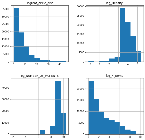
Note the regressor takes a all the data from data frame as they are, so we need to apply the transformations before we build to model as I understand.
# log all the variables
fl17['log_N_Items'] = np.log(fl17['N_Items'])
fl18['log_N_Items'] = np.log(fl18['N_Items'])

# log all the variables
fl17['1*great_circle_dist'] = 1*fl17['great_circle_dist']
fl18['1*great_circle_dist'] = 1*fl18['great_circle_dist']

# Do we need to do the 1-Distance???

fl17['log_NUMBER_OF_PATIENTS'] = np.log(fl17['NUMBER_OF_PATIENTS'])
fl18['log_NUMBER_OF_PATIENTS'] = np.log(fl18['NUMBER_OF_PATIENTS'])

fl17['log_Density'] = np.log(fl17['Density'])
fl18['log_Density'] = np.log(fl18['Density'])

# do the same thing for the complete data

# log all the variables
cfl17['1*great_circle_dist'] = 1*cfl17['great_circle_dist']
cfl18['1*great_circle_dist'] = 1*cfl18['great_circle_dist']

# Do we need to do the 1-Distance???

cfl17['log_NUMBER_OF_PATIENTS'] = np.log(cfl17['NUMBER_OF_PATIENTS'])
cfl18['log_NUMBER_OF_PATIENTS'] = np.log(cfl18['NUMBER_OF_PATIENTS'])

cfl17['log_Density'] = np.log(cfl17['Density'])
cfl18['log_Density'] = np.log(cfl18['Density'])
fl17log = fl17.iloc[:,[77,78,79,80]]
fl18log = fl18.iloc[:,[77,78,79,80]]
fl18log
| log_N_Items | 1*great_circle_dist | log_NUMBER_OF_PATIENTS | log_Density | |
|---|---|---|---|---|
| 0 | 2.079442 | 16.560437 | 9.831723 | 3.602668 |
| 1 | 3.044522 | 0.653229 | 9.831723 | 3.553013 |
| 2 | 8.577159 | 0.983999 | 9.831723 | 3.370474 |
| 3 | 3.258097 | 12.816035 | 9.831723 | 3.355851 |
| 4 | 0.000000 | 20.302017 | 9.831723 | 3.428596 |
| ... | ... | ... | ... | ... |
| 71729 | 0.000000 | 0.973280 | 6.907755 | 5.144711 |
| 71730 | 0.000000 | 1.015876 | 6.907755 | 4.824431 |
| 71731 | 0.693147 | 1.507605 | 6.907755 | 4.806714 |
| 71732 | 1.098612 | 1.739077 | 6.907755 | 4.549942 |
| 71733 | 0.693147 | 1.578409 | 6.907755 | 4.358013 |
71734 rows × 4 columns
fl17log.hist(figsize = (10,10));
Log-normal XGBoost SIM model
Parameters
- booster = ‘dart’
XGBoost mostly combines a huge number of regression trees with a small learning rate. In this situation, trees added early are significant and trees added late are unimportant. Vinayak and Gilad-Bachrach proposed a new method to add dropout techniques from the deep neural net community to boosted trees and reported better results in some situations. Drop trees to solve the over-fitting. Trivial trees (to correct trivial errors) may be prevented. Because of the randomness introduced in the training, expect the following few differences: Training can be slower than gbtree because the random dropout prevents usage of the prediction buffer. The early stop might not be stable, due to the randomness.
Follow here to see all the parameters.
I also found this tutorial which has used the grid search from ‘scikit’ cross validation to test several versions of the model and it's parameters. This comes very handy, as we can instantly find the best performing model in instance. Maybe this can help to explain a bit more about that.
Learning rate = Step size shrinkage used in update to prevents overfitting. After each boosting step, we can directly get the weights of new features, and eta shrinks the feature weights to make the boosting process more conservative.
max_depth = Maximum depth of a tree. Increasing this value will make the model more complex and more likely to overfit. 0 is only accepted in lossguided growing policy when tree_method is set as hist and it indicates no limit on depth. Beware that XGBoost aggressively consumes memory when training a deep tree. Range: [0,∞] (0 is only accepted in lossguided growing policy when tree_method is set as hist)
.
.
.
Note
Below, you can see an example for grid search for the best model within certain parameters. It was very efficient when I was working with the log-normal model only, however, using it within the Poisson version, the model converges after third of all the runs (depends how many options you give it)
# define the training and testing dataset
X_train, y_train = fl17log.loc[:,fl17log.columns != 'log_N_Items'], fl17log.loc[:,['log_N_Items']]
X_test, y_test = fl18log.loc[:,fl18log.columns != 'log_N_Items'], fl18log.loc[:,['log_N_Items']]

# transfer those into matrix as recommended class by in the package
DM_train = xgb.DMatrix(data = X_train,
                       label = y_train)

DM_test =  xgb.DMatrix(data = X_test,
                       label = y_test)

# define the parameters that we want to inspect
gbm_param_grid = {
     'colsample_bytree': np.linspace(0.5, 0.9), # define fairly wide range
     'n_estimators':[15, 20], # try different numbers
     'max_depth': [ 15, 20] # different depths
}

# define the regressor model
gbm = xgb.XGBRegressor(objective = "reg:squarederror", booster = 'dart')

# define the grid search cross validation
grid_mse = GridSearchCV(estimator = gbm, param_grid = gbm_param_grid, scoring = 'neg_mean_squared_error', cv = 5, verbose = 1)

# fit the models and go through all the parameters
grid_mse.fit(X_train, y_train)

# print the best results
print("Best parameters found: ",grid_mse.best_params_)
print("Lowest RMSE found: ", np.sqrt(np.abs(grid_mse.best_score_)))
# define the training and testing dataset
X_train, y_train = fl17log.loc[:,fl17log.columns != 'log_N_Items'], fl17log.loc[:,['log_N_Items']]
X_test, y_test = fl18log.loc[:,fl18log.columns != 'log_N_Items'], fl18log.loc[:,['log_N_Items']]

# define the model (I already tested several version and stacked with the default setting and learning rate 0.4, the grid search is work in progress)
gbm = xgb.XGBRegressor(objective = "reg:squarederror", learning_rate= 0.4).fit(X_train, y_train)
pred = gbm.predict(X_test)

print("Root mean square error for test dataset: {}".format(np.round(np.sqrt(mean_squared_error(np.exp(y_test), np.exp(pred))), 2)))
Root mean square error for test dataset: 949.98
test = pd.DataFrame({"prediction": np.exp(pred), "observed": np.exp(y_test['log_N_Items'])})
lowess = sm.nonparametric.lowess
z = lowess(np.exp(pred).flatten(), np.exp(y_test['log_N_Items']))
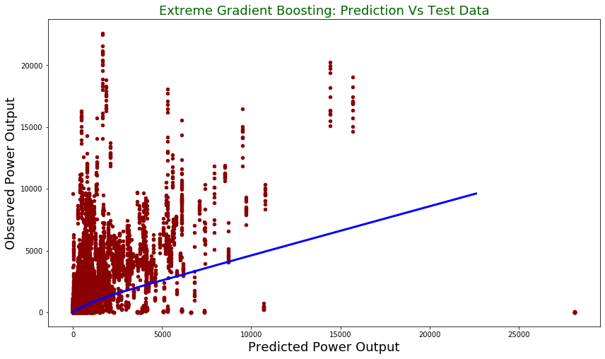
test.plot(figsize = [14,8],
x ="prediction", y = "observed", kind = "scatter", color = 'darkred')
plt.title("Extreme Gradient Boosting: Prediction Vs Test Data", fontsize = 18, color = "darkgreen")
plt.xlabel("Predicted Power Output", fontsize = 18)
plt.ylabel("Observed Power Output", fontsize = 18)
plt.plot(z[:,0], z[:,1], color = "blue", lw= 3)
plt.show()
fl17['log'] =  np.exp(gbm.predict(X_train))

fl18['log'] =  np.exp(gbm.predict(X_test))
Poisson XGBoost SIM model
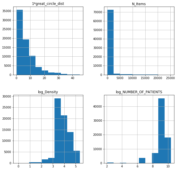
# create new dataset for the Poisson
# this will be logged masses, 1*dist and no change to y
fl17poi = fl17.iloc[:,[6,78,79,80]]
fl18poi = fl18.iloc[:,[6,78,79,80]]
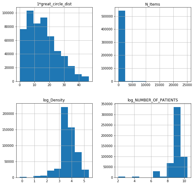
cfl17poi = cfl17.iloc[:,[9,10,11,5]]
cfl18poi = cfl18.iloc[:,[9,10,11,5]]
fl17poi.hist(figsize = (10,10));
cfl17poi.hist(figsize = (10,10));
For published data only
# define the training and testing dataset
X_train2, y_train2 = fl17poi.loc[:,fl17poi.columns != 'N_Items'], fl17poi.loc[:,['N_Items']]
X_test2, y_test2 = fl18poi.loc[:,fl18poi.columns != 'N_Items'], fl18poi.loc[:,['N_Items']]

# define the model
gbm2 = xgb.XGBRegressor(objective = "count:poisson",  learning_rate= 0.4).fit(X_train2, y_train2)
For complete data with all the 0 flows in
# define the training and testing dataset
X_train3, y_train3 = cfl17poi.loc[:,cfl17poi.columns != 'N_Items'], cfl17poi.loc[:,['N_Items']]
X_test3, y_test3 = cfl18poi.loc[:,cfl18poi.columns != 'N_Items'], cfl18poi.loc[:,['N_Items']]

gbm3 = xgb.XGBRegressor(objective = "count:poisson",  learning_rate= 0.4).fit(X_train3, y_train3)
Best parameters found: {‘colsample_bytree’: 0.8, ‘max_depth’: 40, ‘n_estimators’: 30} Lowest RMSE found: 1159.4761503247805
pred2 = gbm2.predict(X_test2)

print("Root mean square error for test dataset: {}".format(np.round(np.sqrt(mean_squared_error(y_test2, pred2)), 2)))

pred3 = gbm3.predict(X_test3)

print("Root mean square error for test dataset: {}".format(np.round(np.sqrt(mean_squared_error(y_test3, pred3)), 2)))
Root mean square error for test dataset: 704.17
Root mean square error for test dataset: 279.73
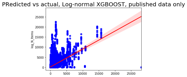
sns.regplot(np.exp(pred), np.exp(y_test['log_N_Items']), color = 'blue',line_kws = {'color':'red'})
plt.title('Predicted vs actual, Log-normal XGBOOST, published data only', fontsize=20);
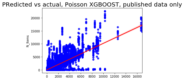
sns.regplot(pred2, y_test2['N_Items'], color = 'blue',line_kws = {'color':'red'})
plt.title('Predicted vs actual, Poisson XGBOOST, published data only', fontsize=20);
sns.regplot(pred3, y_test3['N_Items'], color = 'blue',line_kws = {'color':'red'})
plt.title('Predicted vs actual, Poisson XGBOOST, complete data', fontsize=20);
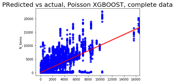
The Poisson seems to be better when using the default parameter setting and learning rate 0.4
We already have the in sample and out of sample predictions from gravity model in the data, so now we need to add the in and out of sample prediction from the XGB model
# published
fl17['xgb'] =  gbm2.predict(X_train2)

fl18['xgb'] =  gbm2.predict(X_test2)

# complete
cfl17['xgb'] =  gbm2.predict(X_train3)

cfl18['xgb'] =  gbm2.predict(X_test3)

fl18.head()
| P_Code | P_Name_x | P_Postcode | D_Code_x | D_Name_x | D_Postcode | N_Items | N_EPSItems | Date | loop | ... | CODE | POSTCODE | NUMBER_OF_PATIENTS | predicted | log_N_Items | 1*great_circle_dist | log_NUMBER_OF_PATIENTS | log_Density | log | xgb | |
|---|---|---|---|---|---|---|---|---|---|---|---|---|---|---|---|---|---|---|---|---|---|
| 0 | L81004 | PORTISHEAD MEDICAL GROUP | BS20 6AQ | FA696 | THE BULLEN HEALTHCARE GROUP LIMITED | BS32 4JT | 8.0 | 0.0 | 2018-01-01 | False | ... | L81004 | BS20 6AQ | 18615 | 0.021203 | 2.079442 | 16.560437 | 9.831723 | 3.602668 | 3.172393 | 2.952730 |
| 1 | L81004 | PORTISHEAD MEDICAL GROUP | BS20 6AQ | FCT35 | LLOYDS PHARMACY LTD | BS20 7QA | 21.0 | 0.0 | 2018-01-01 | False | ... | L81004 | BS20 6AQ | 18615 | 2417.864485 | 3.044522 | 0.653229 | 9.831723 | 3.553013 | 163.713943 | 861.965210 |
| 2 | L81004 | PORTISHEAD MEDICAL GROUP | BS20 6AQ | FDD77 | JOHN WARE LIMITED | BS20 6LT | 5309.0 | 0.0 | 2018-01-01 | False | ... | L81004 | BS20 6AQ | 18615 | 2170.860226 | 8.577159 | 0.983999 | 9.831723 | 3.370474 | 833.031494 | 3730.304199 |
| 3 | L81004 | PORTISHEAD MEDICAL GROUP | BS20 6AQ | FD125 | BOOTS UK LIMITED | BS34 5UP | 26.0 | 0.0 | 2018-01-01 | False | ... | L81004 | BS20 6AQ | 18615 | 0.390401 | 3.258097 | 12.816035 | 9.831723 | 3.355851 | 6.255939 | 5.463578 |
| 4 | L81004 | PORTISHEAD MEDICAL GROUP | BS20 6AQ | FEA59 | LLOYDS PHARMACY LTD | BS16 7AE | 1.0 | 0.0 | 2018-01-01 | False | ... | L81004 | BS20 6AQ | 18615 | 0.001570 | 0.000000 | 20.302017 | 9.831723 | 3.428596 | 3.263482 | 1.575869 |
5 rows × 83 columns
The accuracy measure
Lets organize this into a table;
| R2 Gravity SIM | R2 XGBOOST SIM | RMSE Gravity SIM | RMSE XGBOOST SIM | |
|---|---|---|---|---|
| Models based on published data | PGIr2 | PXIr2 | PGIrs | PXIrs |
| PGOr2 | PXOr2 | PGOrs | PXOrs | |
| Models based on complete data | CGIr2 | CXIr2 | CGIrs | CXIrs |
| CGOr2 | CXOr2 | CGOrs | CXOrs |
# define R2 function
def get_r2_numpy_corrcoef(x, y):
    return np.corrcoef(x, y)[0, 1]**2
# define RMSE function
def rmse(predictions, targets):
    return np.sqrt(((predictions - targets) ** 2).mean())
Other evaluations?
Some is available at Robinsons github, but requires matrices.
See to definition of the Common Part of Commuters measure. Source article
def cpc(actual, predicted):

    # reshape the variables
    predicted = np.reshape(np.array(predicted), (-1, 1))
    actual = np.reshape(np.array(actual),(-1, 1))
    # stack them together
    YYhat = np.hstack([actual, predicted])
    # define sum of the minimym of the predicted var
    NCC = np.sum(np.min(YYhat, axis=1)) # , axis=1
    # number of observations
    N = len(actual)
    # sum of all the actual numbers (reshaped)
    NCY = np.sum(actual)
    # sum of the predicted numbers (reshaped)
    NCYhat = np.sum(predicted)

    numerator = (N * NCC)
    denominator = (NCY + NCYhat)

    return numerator/denominator
$$ \frac{ N_i * \sum \min(ij) }{ \sum_i + \sum_j } $$
def sorensen(actual, predicted):
    # reshape the variables
    predicted = np.reshape(np.array(predicted), (-1, 1))
    actual = np.reshape(np.array(actual),(-1, 1))
    # define length of the variables
    N =  len(actual)
    # stack them together in array
    YYhat = np.hstack([actual, predicted])
    # define 2 times minimum from both
    num = 2.0 * np.min(YYhat, axis=1)
    # define the differnece
    den =  predicted + actual

    return (1.0 / N) * (np.sum(num.reshape((-1, 1)) / den.reshape((-1, 1))))
$$ \frac{1}{N} * \frac{\sum{2 * \min(i,j)} }{j-i} $$
Let's do the result tables again with those measures
| R2 Gravity SIM | R2 XGBOOST SIM | RMSE Gravity SIM | RMSE XGBOOST SIM | CPC Gravity SIM | CPC XGBOOST SIM | SORENSEN I Gravity | SORENSEN I XGBOOST | |
|---|---|---|---|---|---|---|---|---|
| Models based on published data | PGIr2 | PXIr2 | PGIrs | PXIrs | PGIcpc | PXIcpc | PGIsn | PXIsn |
| PGOr2 | PXOr2 | PGOrs | PXOrs | PGOcpc | PXOcpc | PGOsn | PXOsn | |
| Models based on complete data | CGIr2 | CXIr2 | CGIrs | CXIrs | CGIcpc | CXIcpc | CGIsn | CXIsn |
| CGOr2 | CXOr2 | CGOrs | CXOrs | CGOcpc | CXOcpc | CGOsn | CXOsn |
# R2
# published data
PGIr2 = round(get_r2_numpy_corrcoef(fl17['N_Items'], fl17['yhat']),3)
PGOr2 = round(get_r2_numpy_corrcoef(fl18['N_Items'], fl18['predicted']),3)

PXIr2 = round(get_r2_numpy_corrcoef(fl17['N_Items'], fl17['xgb']),3)
PXOr2 = round(get_r2_numpy_corrcoef(fl18['N_Items'], fl18['xgb']),3)

# complete data
CGIr2 = round(get_r2_numpy_corrcoef(cfl17['N_Items'], cfl17['yhat']),3)
CGOr2 = round(get_r2_numpy_corrcoef(cfl18['N_Items'], cfl18['predicted']),3)

CXIr2 = round(get_r2_numpy_corrcoef(cfl17['N_Items'], cfl17['xgb']),3)
CXOr2 = round(get_r2_numpy_corrcoef(cfl18['N_Items'], cfl18['xgb']),3)
# RMSE

PGIrs = round(rmse(fl17['N_Items'], fl17['yhat']),1)
PGOrs = round(rmse(fl18['N_Items'], fl18['predicted']),1)

PXIrs = round(rmse(fl17['N_Items'], fl17['xgb']),1)
PXOrs = round(rmse(fl18['N_Items'], fl18['xgb']),1)

CGIrs = round(rmse(cfl17['N_Items'], cfl17['yhat']),1)
CGOrs = round(rmse(cfl18['N_Items'], cfl18['predicted']),1)

CXIrs = round(rmse(cfl17['N_Items'], cfl17['xgb']),1)
CXOrs = round(rmse(cfl18['N_Items'], cfl18['xgb']),1)
# CPC

PGIcpc = round(cpc(fl17['N_Items'], fl17['yhat']),1)
PGOcpc = round(cpc(fl18['N_Items'], fl18['predicted']),1)

PXIcpc = round(cpc(fl17['N_Items'], fl17['xgb']),1)
PXOcpc = round(cpc(fl18['N_Items'], fl18['xgb']),1)

CGIcpc = round(cpc(cfl17['N_Items'], cfl17['yhat']),1)
CGOcpc = round(cpc(cfl18['N_Items'], cfl18['predicted']),1)

CXIcpc = round(cpc(cfl17['N_Items'], cfl17['xgb']),1)
CXOcpc = round(cpc(cfl18['N_Items'], cfl18['xgb']),1)
# Sorensen

PGIsn = round(sorensen(fl17['N_Items'], fl17['yhat']),3)
PGOsn = round(sorensen(fl18['N_Items'], fl18['predicted']),3)

PXIsn = round(sorensen(fl17['N_Items'], fl17['xgb']),3)
PXOsn = round(sorensen(fl18['N_Items'], fl18['xgb']),3)

CGIsn = round(sorensen(cfl17['N_Items'], cfl17['yhat']),3)
CGOsn = round(sorensen(cfl18['N_Items'], cfl18['predicted']),3)

CXIsn = round(sorensen(cfl17['N_Items'], cfl17['xgb']),3)
CXOsn = round(sorensen(cfl18['N_Items'], cfl18['xgb']),3)
# everything for the log-normal model
LXIr2 = round(get_r2_numpy_corrcoef(fl17['N_Items'], fl17['log']),3)
LXOr2 = round(get_r2_numpy_corrcoef(fl18['N_Items'], fl18['log']),3)

LXIrs = round(rmse(fl17['N_Items'], fl17['log']),1)
LXOrs = round(rmse(fl18['N_Items'], fl18['log']),1)

LXIcpc = round(cpc(fl17['N_Items'], fl17['log']),1)
LXOcpc = round(cpc(fl18['N_Items'], fl18['log']),1)

LXIsn = round(sorensen(fl17['N_Items'], fl17['log']),3)
LXOsn = round(sorensen(fl18['N_Items'], fl18['log']),3)
model_name = ['In-sample','Out-sample']
mG = [PGIr2, PGOr2]
mX = [PXIr2, PXOr2]
mF = [PGIrs, PGOrs]
mH = [PXIrs, PXOrs]
mD1 = [PGIcpc, PGOcpc]
mD2 = [PXIcpc, PXOcpc]
mK1 = [PGIsn, PGOsn]
mK2 = [PXIsn, PXOsn]

cols = {'Poisson models based on published data': model_name,'R2 Gravity SIM': mG, 'R2 XGBOOST SIM': mX, 'RMSE Gravity SIM': mF, 'RMSE XGBOOST SIM': mH, 'CPC Gravity SIM': mD1,
      'CPC XGBOOST SIM': mD2,  'SORENSEN I Gravity': mK1, 'SORENSEN I XGBOOST': mK2}

table_published = pd.DataFrame(cols).set_index('Poisson models based on published data')
model_name = ['In-sample','Out-sample']
G = [CGIr2, CGOr2]
X = [CXIr2, CXOr2]
mF = [CGIrs, CGOrs]
mH = [CXIrs, CXOrs]
mD1 = [CGIcpc, CGOcpc]
mD2 = [CXIcpc, CXOcpc]
mK1 = [CGIsn, CGOsn]
mK2 = [CXIsn, CXOsn]

cols = {'Poisson models based on complete data': model_name,'R2 Gravity SIM': G, 'R2 XGBOOST SIM': X, 'RMSE Gravity SIM': mF, 'RMSE XGBOOST SIM': mH,  'CPC Gravity SIM': mD1,
      'CPC XGBOOST SIM': mD2,  'SORENSEN I Gravity': mK1, 'SORENSEN I XGBOOST': mK2}

table_complete = pd.DataFrame(cols).set_index('Poisson models based on complete data')
NA = 'NA'
model_name = ['In-sample','Out-sample']
mG = [NA, NA]
mX = [LXIr2, LXOr2]
mF = [NA, NA]
mH = [LXIrs, LXOrs]
mD1 = [NA, NA]
mD2 = [LXIcpc, LXOcpc]
mK1 = [NA, NA]
mK2 = [LXIsn, LXOsn]

cols = {'Log-normal models based on published data': model_name,'R2 Gravity SIM': mG, 'R2 XGBOOST SIM': mX, 'RMSE Gravity SIM': mF, 'RMSE XGBOOST SIM': mH, 'CPC Gravity SIM': mD1,
      'CPC XGBOOST SIM': mD2,  'SORENSEN I Gravity': mK1, 'SORENSEN I XGBOOST': mK2}

table_log = pd.DataFrame(cols).set_index('Log-normal models based on published data')
table_log
| R2 Gravity SIM | R2 XGBOOST SIM | RMSE Gravity SIM | RMSE XGBOOST SIM | CPC Gravity SIM | CPC XGBOOST SIM | SORENSEN I Gravity | SORENSEN I XGBOOST | |
|---|---|---|---|---|---|---|---|---|
| Log-normal models based on published data | ||||||||
| In-sample | NA | 0.560 | NA | 809.9 | NA | 25504.1 | NA | 0.686 |
| Out-sample | NA | 0.381 | NA | 950.0 | NA | 21690.5 | NA | 0.620 |
# models based on published data only
table_published
| R2 Gravity SIM | R2 XGBOOST SIM | RMSE Gravity SIM | RMSE XGBOOST SIM | CPC Gravity SIM | CPC XGBOOST SIM | SORENSEN I Gravity | SORENSEN I XGBOOST | |
|---|---|---|---|---|---|---|---|---|
| Poisson models based on published data | ||||||||
| In-sample | 0.321 | 0.736 | 976.2 | 611.1 | 17813.1 | 27736.8 | 0.318 | 0.513 |
| Out-sample | 0.330 | 0.653 | 981.4 | 704.2 | 17207.5 | 24790.0 | 0.314 | 0.490 |
# models based on complete data with all the zero flows included
table_complete
| R2 Gravity SIM | R2 XGBOOST SIM | RMSE Gravity SIM | RMSE XGBOOST SIM | CPC Gravity SIM | CPC XGBOOST SIM | SORENSEN I Gravity | SORENSEN I XGBOOST | |
|---|---|---|---|---|---|---|---|---|
| Poisson models based on complete data | ||||||||
| In-sample | 0.287 | 0.691 | 380.6 | 249.9 | 106667.5 | 168990.5 | 0.045 | 0.070 |
| Out-sample | 0.297 | 0.605 | 385.3 | 288.8 | 100976.7 | 145788.9 | 0.046 | 0.068 |
x = table_log.append(table_published)
x = x.append(table_complete)
x['model_type'] = ['log-normal', 'log-normal', 'Poisson', 'Poisson', 'Poisson', 'Poisson']
x['data_type'] = ['published_only', 'published_only', 'published_only', 'published_only', 'complete', 'complete']
x['CV'] = ['In-sample', 'Out-sample','In-sample', 'Out-sample','In-sample', 'Out-sample']
x = x.set_index(['model_type', 'data_type'])
x
| R2 Gravity SIM | R2 XGBOOST SIM | RMSE Gravity SIM | RMSE XGBOOST SIM | CPC Gravity SIM | CPC XGBOOST SIM | SORENSEN I Gravity | SORENSEN I XGBOOST | CV | ||
|---|---|---|---|---|---|---|---|---|---|---|
| model_type | data_type | |||||||||
| log-normal | published_only | NA | 0.560 | NA | 809.9 | NA | 25504.1 | NA | 0.686 | In-sample |
| published_only | NA | 0.381 | NA | 950.0 | NA | 21690.5 | NA | 0.620 | Out-sample | |
| Poisson | published_only | 0.321 | 0.736 | 976.2 | 611.1 | 17813.1 | 27736.8 | 0.318 | 0.513 | In-sample |
| published_only | 0.33 | 0.653 | 981.4 | 704.2 | 17207.5 | 24790.0 | 0.314 | 0.490 | Out-sample | |
| complete | 0.287 | 0.691 | 380.6 | 249.9 | 106668 | 168990.5 | 0.045 | 0.070 | In-sample | |
| complete | 0.297 | 0.605 | 385.3 | 288.8 | 100977 | 145788.9 | 0.046 | 0.068 | Out-sample |
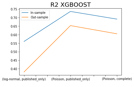
x.iloc[[0,2,4],:]['R2 XGBOOST SIM'].plot()
x.iloc[[1,3,5],:]['R2 XGBOOST SIM'].plot()
plt.title('R2 XGBOOST', fontsize=20)
plt.legend(['In-sample', 'Out-sample'])
plt.xlabel(' ');
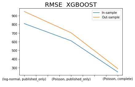
x.iloc[[0,2,4],:]['RMSE XGBOOST SIM'].plot()
x.iloc[[1,3,5],:]['RMSE XGBOOST SIM'].plot()
plt.title('RMSE  XGBOOST', fontsize=20)
plt.legend(['In-sample', 'Out-sample'])
plt.xlabel(' ');
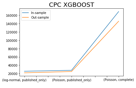
x.iloc[[0,2,4],:]['CPC XGBOOST SIM'].plot()
x.iloc[[1,3,5],:]['CPC XGBOOST SIM'].plot()
plt.title('CPC XGBOOST', fontsize=20)
plt.legend(['In-sample', 'Out-sample'])
plt.xlabel(' ');
x.iloc[[0,2,4],:]['SORENSEN I XGBOOST'].plot()
x.iloc[[1,3,5],:]['SORENSEN I XGBOOST'].plot()
plt.title('SORENSEN XGBOOST', fontsize=20)
plt.legend(['In-sample', 'Out-sample'])
plt.xlabel(' ');
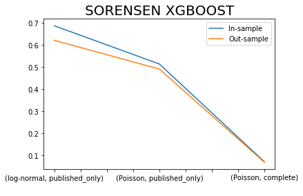
Sorensen similarity Index is bounded between values of 0 and 1 with values closer to 1 indicating a better model fit.
How come that the complete dataset has exceptionally low index, because of the zero issue?
cfl17.loc[:,['N_Items', 'xgb']]
| N_Items | xgb | |
|---|---|---|
| 0 | 130.0 | 11.200489 |
| 1 | 39.0 | 7.248779 |
| 2 | 12.0 | 3.174812 |
| 3 | 661.0 | 861.965210 |
| 4 | 4058.0 | 3730.304199 |
| ... | ... | ... |
| 543739 | 0.0 | 8.880725 |
| 543740 | 0.0 | 5.127942 |
| 543741 | 0.0 | 5.786361 |
| 543742 | 0.0 | 7.492306 |
| 543743 | 0.0 | 18.535973 |
543744 rows × 2 columns
Prob it is caused by the excessive zeros, we would probably need to introduce an ensemble model to deal with it.
Some other is available from Tylor Oshan He has CPC as well as Sorensen index