Sensitivity analysis
Can we safely change a value of variable without casing harm? How is it going to affect the model results?
Load the data and the libraries
import pandas as pd
import os
import numpy as np
import glob
import geopandas as gpd
from shapely.geometry import Point
import matplotlib.pyplot as plt
import datetime as dt
import seaborn as sns
import plotly.express as px
import itertools
from scipy import stats
import sys
sys.path.append('/Users/toshan/dev/pysal/pysal/contrib/spint')
from spint.gravity import Gravity, BaseGravity
import spint.gravity
#from utils import sorensen
import statsmodels.formula.api as smf
from statsmodels.api import families as families
wgs84 = {'init':'EPSG:4326'}
bng = {'init':'EPSG:27700'}
file = './../../data/NHS/working/year_data_flow/flow_2018.csv'
fl18 = pd.read_csv(file, index_col=None)

file = './../../data/NHS/working/year_data_flow/flow_2017.csv'
fl17 = pd.read_csv(file, index_col=None)

file = './../../data/NHS/working/year_data_flow/flow_2016.csv'
fl16 = pd.read_csv(file, index_col=None)

file = './../../data/NHS/working/year_data_flow/flow_2015.csv'
fl15 = pd.read_csv(file, index_col=None)

# plot the top of the table
fl18.head()
| P_Code | P_Name_x | P_Postcode | D_Code_x | D_Name_x | D_Postcode | N_Items | N_EPSItems | Date | loop | ... | P_Name | P_full_address_y | P_Status_Code_y | P_Sub_type_y | P_Setting_y | P_X_y | P_Y_y | CODE | POSTCODE | NUMBER_OF_PATIENTS | |
|---|---|---|---|---|---|---|---|---|---|---|---|---|---|---|---|---|---|---|---|---|---|
| 0 | L81004 | PORTISHEAD MEDICAL GROUP | BS20 6AQ | FA696 | THE BULLEN HEALTHCARE GROUP LIMITED | BS32 4JT | 8.0 | 0.0 | 2018-01-01 | False | ... | PORTISHEAD MEDICAL GROUP | PORTISHEAD MEDICAL GROUP,PORTISHEAD MEDICAL GR... | A | B | 4 | -2.767318 | 51.482805 | L81004 | BS20 6AQ | 18615 |
| 1 | L81004 | PORTISHEAD MEDICAL GROUP | BS20 6AQ | FCT35 | LLOYDS PHARMACY LTD | BS20 7QA | 21.0 | 0.0 | 2018-01-01 | False | ... | PORTISHEAD MEDICAL GROUP | PORTISHEAD MEDICAL GROUP,PORTISHEAD MEDICAL GR... | A | B | 4 | -2.767318 | 51.482805 | L81004 | BS20 6AQ | 18615 |
| 2 | L81004 | PORTISHEAD MEDICAL GROUP | BS20 6AQ | FDD77 | JOHN WARE LIMITED | BS20 6LT | 5309.0 | 0.0 | 2018-01-01 | False | ... | PORTISHEAD MEDICAL GROUP | PORTISHEAD MEDICAL GROUP,PORTISHEAD MEDICAL GR... | A | B | 4 | -2.767318 | 51.482805 | L81004 | BS20 6AQ | 18615 |
| 3 | L81004 | PORTISHEAD MEDICAL GROUP | BS20 6AQ | FD125 | BOOTS UK LIMITED | BS34 5UP | 26.0 | 0.0 | 2018-01-01 | False | ... | PORTISHEAD MEDICAL GROUP | PORTISHEAD MEDICAL GROUP,PORTISHEAD MEDICAL GR... | A | B | 4 | -2.767318 | 51.482805 | L81004 | BS20 6AQ | 18615 |
| 4 | L81004 | PORTISHEAD MEDICAL GROUP | BS20 6AQ | FEA59 | LLOYDS PHARMACY LTD | BS16 7AE | 1.0 | 0.0 | 2018-01-01 | False | ... | PORTISHEAD MEDICAL GROUP | PORTISHEAD MEDICAL GROUP,PORTISHEAD MEDICAL GR... | A | B | 4 | -2.767318 | 51.482805 | L81004 | BS20 6AQ | 18615 |
5 rows × 76 columns
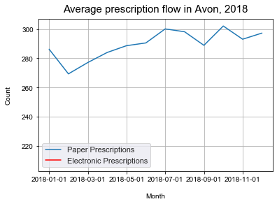
Look ate the time series of the prescription flow
monthly = fl18.set_index('Date')
monthly = monthly.groupby(monthly.index).mean()
cols = ["N_EPSItems"]
monthly['N_EPSItems'] = monthly['N_EPSItems'].replace({0:np.nan})
ax = plt.axes()
sns.set(rc={'figure.figsize':(20, 6)})
monthly['N_Items'].plot()
monthly['N_EPSItems'].plot(color = 'red')
#set legend
plt.legend(labels=['Paper Prescriptions', 'Electronic Prescriptions'])
# Add axis and chart labels.
ax.set_xlabel('Month', labelpad=15)
ax.set_ylabel('Count', labelpad=15)
ax.set_title('Average prescription flow in Avon, 2018', pad=10, size = 15)
# sort out thex axes
#plt.xticks([ 8, 20, 32, 44, 56, 68, 80 ], ('December 2012', 'December 2013', 'December 2014', 'December 2015', 'December 2016', 'December 2017', 'December 2018'),rotation=20);
#plt.xticks([ 0, 12, 24, 36, 48, 60, 72], ('January 2013', 'January 2014', 'January 2015', 'January 2016', 'January 2017', 'January 2018', 'January 2019'),rotation=20);
Text(0.5, 1.0, 'Average prescription flow in Avon, 2018')
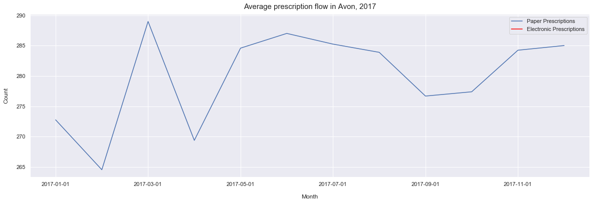
monthly = fl17.set_index('Date')
monthly = monthly.groupby(monthly.index).mean()
cols = ["N_EPSItems"]
monthly['N_EPSItems'] = monthly['N_EPSItems'].replace({0:np.nan})
ax = plt.axes()
sns.set(rc={'figure.figsize':(20, 6)})
monthly['N_Items'].plot()
monthly['N_EPSItems'].plot(color = 'red')
#set legend
plt.legend(labels=['Paper Prescriptions', 'Electronic Prescriptions'])
# Add axis and chart labels.
ax.set_xlabel('Month', labelpad=15)
ax.set_ylabel('Count', labelpad=15)
ax.set_title('Average prescription flow in Avon, 2017', pad=10, size = 15)
# sort out thex axes
#plt.xticks([ 8, 20, 32, 44, 56, 68, 80 ], ('December 2012', 'December 2013', 'December 2014', 'December 2015', 'December 2016', 'December 2017', 'December 2018'),rotation=20);
#plt.xticks([ 0, 12, 24, 36, 48, 60, 72], ('January 2013', 'January 2014', 'January 2015', 'January 2016', 'January 2017', 'January 2018', 'January 2019'),rotation=20);
Text(0.5, 1.0, 'Average prescription flow in Avon, 2017')
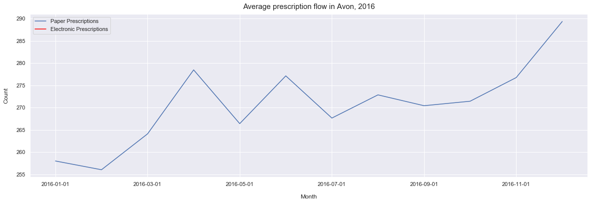
monthly = fl16.set_index('Date')
monthly = monthly.groupby(monthly.index).mean()
cols = ["N_EPSItems"]
monthly['N_EPSItems'] = monthly['N_EPSItems'].replace({0:np.nan})
ax = plt.axes()
sns.set(rc={'figure.figsize':(20, 6)})
monthly['N_Items'].plot()
monthly['N_EPSItems'].plot(color = 'red')
#set legend
plt.legend(labels=['Paper Prescriptions', 'Electronic Prescriptions'])
# Add axis and chart labels.
ax.set_xlabel('Month', labelpad=15)
ax.set_ylabel('Count', labelpad=15)
ax.set_title('Average prescription flow in Avon, 2016', pad=10, size = 15)
# sort out thex axes
#plt.xticks([ 8, 20, 32, 44, 56, 68, 80 ], ('December 2012', 'December 2013', 'December 2014', 'December 2015', 'December 2016', 'December 2017', 'December 2018'),rotation=20);
#plt.xticks([ 0, 12, 24, 36, 48, 60, 72], ('January 2013', 'January 2014', 'January 2015', 'January 2016', 'January 2017', 'January 2018', 'January 2019'),rotation=20);
Text(0.5, 1.0, 'Average prescription flow in Avon, 2016')
monthly = fl15.set_index('Date')
monthly = monthly.groupby(monthly.index).mean()
cols = ["N_EPSItems"]
monthly['N_EPSItems'] = monthly['N_EPSItems'].replace({0:np.nan})
ax = plt.axes()
sns.set(rc={'figure.figsize':(20, 6)})
monthly['N_Items'].plot()
monthly['N_EPSItems'].plot(color = 'red')
#set legend
plt.legend(labels=['Paper Prescriptions', 'Electronic Prescriptions'])
# Add axis and chart labels.
ax.set_xlabel('Month', labelpad=15)
ax.set_ylabel('Count', labelpad=15)
ax.set_title('Average prescription flow in Avon, 2015', pad=10, size = 15)
# sort out thex axes
#plt.xticks([ 8, 20, 32, 44, 56, 68, 80 ], ('December 2012', 'December 2013', 'December 2014', 'December 2015', 'December 2016', 'December 2017', 'December 2018'),rotation=20);
#plt.xticks([ 0, 12, 24, 36, 48, 60, 72], ('January 2013', 'January 2014', 'January 2015', 'January 2016', 'January 2017', 'January 2018', 'January 2019'),rotation=20);
Text(0.5, 1.0, 'Average prescription flow in Avon, 2015')
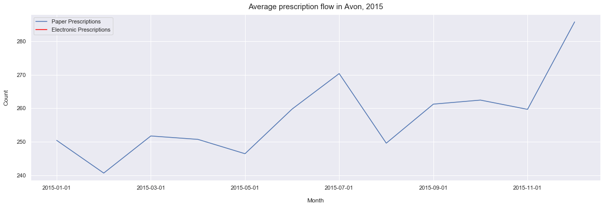
From this we can see the the average number of prescriptions is slowly increasing over time. However, we can also see that the years 2017 and 2018 are fairly stable years in compare with the 2016 and 2015 which has some significant fluctations in the average prescribing.
Look at the variables in 2017 and 2018
plt.figure(figsize = [15,10])
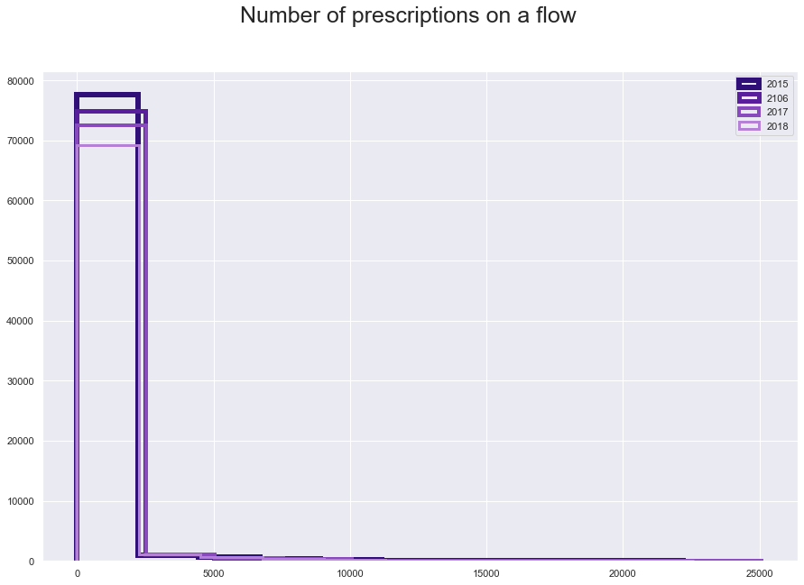
plt.suptitle("Number of prescriptions on a flow", fontsize=25)
plt.hist(fl15['N_Items'], histtype='step', linewidth=6, color = '#310F78')
plt.hist(fl16['N_Items'], histtype='step', linewidth=5, color = '#581E9B')
plt.hist(fl17['N_Items'], histtype='step', linewidth=4, color = '#894ABD')
plt.hist(fl18['N_Items'], histtype='step',linewidth=3, color = '#B581D6')
plt.legend(labels=['2015', '2106', '2017', '2018']);
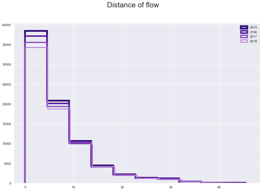
plt.figure(figsize = [15,10])
plt.suptitle("Distance of flow", fontsize=25)
plt.hist(fl15['great_circle_dist'], histtype='step', linewidth=6 , color = '#310F78')
plt.hist(fl16['great_circle_dist'], histtype='step', linewidth=5 ,color = '#581E9B')
plt.hist(fl17['great_circle_dist'], histtype='step', linewidth=4,color = '#894ABD' )
plt.hist(fl18['great_circle_dist'], histtype='step',linewidth=3 ,color = '#B581D6')
plt.legend(labels=['2015', '2106', '2017', '2018']);
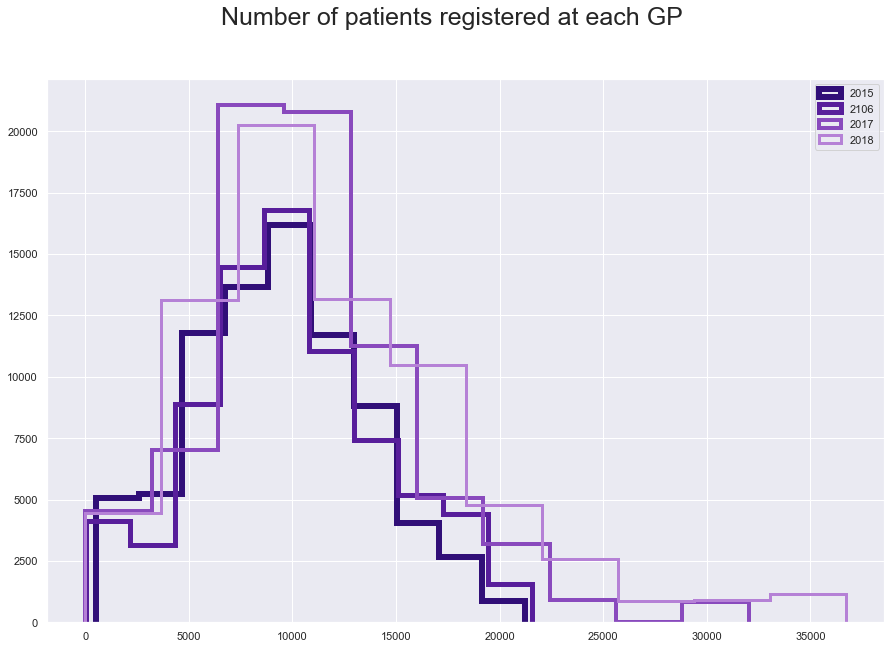
plt.figure(figsize = [15,10])
plt.suptitle("Number of patients registered at each GP", fontsize=25)
plt.hist(fl15['NUMBER_OF_PATIENTS'], histtype='step', linewidth=6 , color = '#310F78')
plt.hist(fl16['NUMBER_OF_PATIENTS'], histtype='step', linewidth=5 ,color = '#581E9B')
plt.hist(fl17['NUMBER_OF_PATIENTS'], histtype='step', linewidth=4,color = '#894ABD' )
plt.hist(fl18['NUMBER_OF_PATIENTS'], histtype='step',linewidth=3 ,color = '#B581D6')
plt.legend(labels=['2015', '2106', '2017', '2018']);
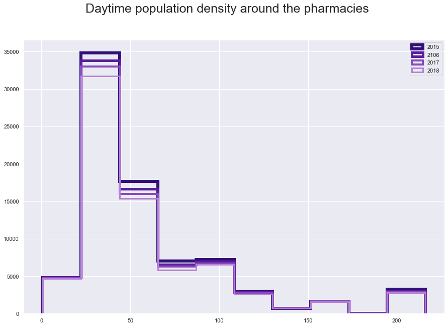
plt.figure(figsize = [15,10])
plt.suptitle("Daytime population density around the pharmacies", fontsize=25)
plt.hist(fl15['Density'], histtype='step', linewidth=6 , color = '#310F78')
plt.hist(fl16['Density'], histtype='step', linewidth=5,color = '#581E9B' )
plt.hist(fl17['Density'], histtype='step', linewidth=4,color = '#894ABD' )
plt.hist(fl18['Density'], histtype='step',linewidth=3,color = '#B581D6' )
plt.legend(labels=['2015', '2106', '2017', '2018']);
fl15.iloc[:,[6, 48, 76, 65]].describe()
| N_Items | great_circle_dist | NUMBER_OF_PATIENTS | Density | |
|---|---|---|---|---|
| count | 79975.000000 | 79975.000000 | 79975.000000 | 79975.000000 |
| mean | 257.286565 | 6.904360 | 9345.992135 | 59.599734 |
| std | 1112.177455 | 6.579699 | 4298.057099 | 43.362001 |
| min | 1.000000 | 0.000000 | 530.000000 | 0.833333 |
| 25% | 2.000000 | 2.425812 | 6615.000000 | 33.543636 |
| 50% | 6.000000 | 4.768408 | 9454.000000 | 44.194643 |
| 75% | 53.000000 | 9.289434 | 12104.000000 | 72.205556 |
| max | 22311.000000 | 45.367788 | 21238.000000 | 216.139024 |
fl16.iloc[:,[6, 48, 76, 65]].describe()
| N_Items | great_circle_dist | NUMBER_OF_PATIENTS | Density | |
|---|---|---|---|---|
| count | 77099.000000 | 77099.000000 | 77099.000000 | 77099.000000 |
| mean | 270.637596 | 6.881413 | 9919.814628 | 59.580914 |
| std | 1162.624077 | 6.576676 | 4604.358012 | 43.440339 |
| min | 1.000000 | 0.000000 | 16.000000 | 0.833333 |
| 25% | 2.000000 | 2.434314 | 6752.000000 | 33.543636 |
| 50% | 6.000000 | 4.752313 | 9669.000000 | 43.840426 |
| 75% | 56.000000 | 9.188920 | 12805.000000 | 72.205556 |
| max | 25077.000000 | 45.334545 | 21588.000000 | 216.139024 |
fl17.iloc[:,[6, 48, 75, 65]].describe()
| N_Items | great_circle_dist | NUMBER_OF_PATIENTS | Density | |
|---|---|---|---|---|
| count | 74668.000000 | 74668.000000 | 74668.000000 | 74668.000000 |
| mean | 280.026316 | 6.920288 | 10663.137542 | 59.422628 |
| std | 1181.619314 | 6.493172 | 5293.086633 | 43.452671 |
| min | 1.000000 | 0.000000 | 8.000000 | 0.833333 |
| 25% | 2.000000 | 2.465416 | 7117.000000 | 33.077419 |
| 50% | 7.000000 | 4.828210 | 10191.000000 | 43.243548 |
| 75% | 62.000000 | 9.427593 | 13344.000000 | 72.205556 |
| max | 25161.000000 | 45.334545 | 32033.000000 | 216.139024 |
fl18.iloc[:,[6, 48, 75, 65]].describe()
| N_Items | great_circle_dist | NUMBER_OF_PATIENTS | Density | |
|---|---|---|---|---|
| count | 71734.000000 | 71734.000000 | 71734.000000 | 71734.000000 |
| mean | 289.512031 | 6.958728 | 11863.355564 | 59.193355 |
| std | 1195.221113 | 6.490907 | 6718.805457 | 43.402032 |
| min | 1.000000 | 0.000000 | 5.000000 | 0.833333 |
| 25% | 2.000000 | 2.513705 | 7367.000000 | 32.875000 |
| 50% | 7.000000 | 4.851604 | 10520.000000 | 43.243548 |
| 75% | 58.000000 | 9.491935 | 15562.000000 | 72.205556 |
| max | 22604.000000 | 46.139331 | 36737.000000 | 216.139024 |
fl18['great_circle_dist'].value_counts(normalize = True)
0.000000     0.026055
2.125845     0.000934
3.936654     0.000822
23.579141    0.000767
1.719747     0.000711
               ...
24.894594    0.000014
30.107116    0.000014
5.912814     0.000014
22.904229    0.000014
6.988423     0.000014
Name: great_circle_dist, Length: 11299, dtype: float64
The only variable we might have an issue is the distance, which has a lowest value zero. The zero belong to 2.6% o the data which is significant but should not be a big issue to change.
Also we can notice that number of patients registered at GP is very differnt for the 2017 than for the other years, why is it so?
Let's have a look into it
Examining the ‘Number of patients Registered at GP’
The reson for the difference in the distributions is complex.
In 2016, NHS started to joining surgeries into a groups(health group, health centres with more branches,…). In 2016, each branch was recorded as row and each branch had its own number of patients. For example, those are records for all the branches of Fireclay Health Group (fictional). Each surgery has recorded of registered patients that is unique for each surgery and is more or less the same as the number of patients in 2015. None of the data contain any record of if the surgeries belong to group and which group could it be. This information is not availiable in the data, or anywhere else to my knowledge.
| ID | Name | Number of Patients |
|---|---|---|
| 1 | Churchroad surgery | 2000 |
| 2 | Barewell surgery | 3000 |
| 3 | Longwell surgery | 4000 |
| 4 | Bond street surgery | 6000 |
In 2017 they records show the number of patients for each the branch as well as for the whole group, but this is actually recorded as one of the branches. This essentially means that the patients are doubled or multiplied in the data, in other words, some patients are counted twice in the data.
| ID | Name | Number of Patients |
|---|---|---|
| 1 | Churchroad surgery | 2000 |
| 2 | Barewell surgery | 3000 |
| 3 | Longwell surgery | 4000 |
| 4 | Bond street surgery | 15000 |
This continue to 2018 January, but by the July the NHS changed the way they shared published the numbers and corrceted themselves. They now only post the grouped number of patients for all the branches, so the patients should not appear multiple times in the data. This has one issue though, although the little branches exists, the record will show not the group name but the biggest branch with all the patients and the little branches (although still existing) are not present in the data.
| ID | Name | Number of Patients |
|---|---|---|
| 4 | Bond street surgery | 15000 |
Question is, do we need to do something with that??
Adding low value to all flows
for i in np.linspace(0.001, 1 , num = 10):
    plt.hist(x= (np.log(fl18['great_circle_dist'] + i)), color='g')
    plt.legend(labels=[i])
    plt.figure()
    plt.show();
Impact on the model
We need to find out what is going to be less impactfull
- Zero substitution only
or
- Add small amount to all variables
I will be handling many variables now, those datasets with 1. will have subscript _sub and those with 2 will have subscript _add
For the Power law models
| what | how | value | 2015 | 2016 | 2017 | 2018 |
|---|---|---|---|---|---|---|
| Model Power | substituted | 0.001 | mps531 | mps631 | mps731 | mps831 |
| Model Power | substituted | 0.01 | mps521 | mps621 | mps721 | mps821 |
| Model Power | substituted | 0.1 | mps511 | mps611 | mps711 | mps811 |
| Model Power | substituted | 1 | mps501 | mps601 | mps701 | mps801 |
| Model Power | added | 0.001 | mpa531 | mpa631 | mpa731 | mpa831 |
| Model Power | added | 0.01 | mpa521 | mpa621 | mpa721 | mpa821 |
| Model Power | added | 0.1 | mpa511 | mpa611 | mpa711 | mpa811 |
| Model Power | added | 1 | mpa501 | mpa601 | mpa701 | mpa801 |
For the Exponential law models
| what | how | value | 2015 | 2016 | 2017 | 2018 |
|---|---|---|---|---|---|---|
| Model Exponential | substituted | 0.001 | mes531 | mes631 | mes731 | mes831 |
| Model Exponential | substituted | 0.01 | mes521 | mes621 | mes721 | mes821 |
| Model Exponential | substituted | 0.1 | mes511 | mes611 | mes711 | mes811 |
| Model Exponential | substituted | 1 | mes501 | mes601 | mes701 | mes801 |
| Model Exponential | added | 0.001 | mea531 | mea631 | mea731 | mea831 |
| Model Exponential | added | 0.01 | mea521 | mea621 | mea721 | mea821 |
| Model Exponential | added | 0.1 | mea511 | mea611 | mea711 | mea811 |
| Model Exponential | added | 1 | mea501 | mea601 | mea701 | mea801 |
Build the data for the substitute
fl180 = fl18.iloc[:,[6,8, 48, 75, 65]]
fl170 = fl17.iloc[:,[6,8, 48, 75, 65]]
fl160 = fl16.iloc[:,[6,8, 48, 76, 65]]
fl150 = fl15.iloc[:,[6,8, 48, 76, 65]]
# 0.001
fl180['dist_adjusted_0001']= fl180['great_circle_dist'].mask(fl180['great_circle_dist'] == 0, 0.001)
fl170['dist_adjusted_0001'] = fl170['great_circle_dist'].mask(fl170['great_circle_dist'] == 0, 0.001)
fl160['dist_adjusted_0001'] = fl160['great_circle_dist'].mask(fl160['great_circle_dist'] == 0, 0.001)
fl150['dist_adjusted_0001'] = fl150['great_circle_dist'].mask(fl150['great_circle_dist'] == 0, 0.001)
# 0.01
fl180['dist_adjusted_001']= fl180['great_circle_dist'].mask(fl180['great_circle_dist'] == 0, 0.01)
fl170['dist_adjusted_001'] = fl170['great_circle_dist'].mask(fl170['great_circle_dist'] == 0, 0.01)
fl160['dist_adjusted_001'] = fl160['great_circle_dist'].mask(fl160['great_circle_dist'] == 0, 0.01)
fl150['dist_adjusted_001'] = fl150['great_circle_dist'].mask(fl150['great_circle_dist'] == 0, 0.01)
# 0.1
fl180['dist_adjusted_01']= fl180['great_circle_dist'].mask(fl180['great_circle_dist'] == 0, 0.1)
fl170['dist_adjusted_01'] = fl170['great_circle_dist'].mask(fl170['great_circle_dist'] == 0, 0.1)
fl160['dist_adjusted_01'] = fl160['great_circle_dist'].mask(fl160['great_circle_dist'] == 0, 0.1)
fl150['dist_adjusted_01'] = fl150['great_circle_dist'].mask(fl150['great_circle_dist'] == 0, 0.1)
# 1
fl180['dist_adjusted_1']= fl180['great_circle_dist'].mask(fl180['great_circle_dist'] == 0, 1)
fl170['dist_adjusted_1'] = fl170['great_circle_dist'].mask(fl170['great_circle_dist'] == 0, 1)
fl160['dist_adjusted_1'] = fl160['great_circle_dist'].mask(fl160['great_circle_dist'] == 0, 1)
fl150['dist_adjusted_1'] = fl150['great_circle_dist'].mask(fl150['great_circle_dist'] == 0, 1)
plt.figure(figsize = [15,10])
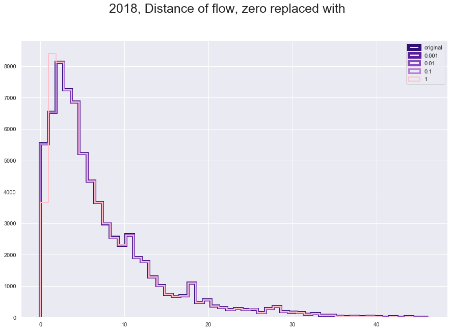
plt.suptitle("2018, Distance of flow, zero replaced with", fontsize=25)
plt.hist(fl180['great_circle_dist'], histtype='step', linewidth=6 , color = '#310F78', bins = 50)
plt.hist(fl180['dist_adjusted_0001'], histtype='step', linewidth=5 ,color = '#581E9B', bins = 50)
plt.hist(fl180['dist_adjusted_001'], histtype='step', linewidth=4,color = '#894ABD' , bins = 50)
plt.hist(fl180['dist_adjusted_01'], histtype='step',linewidth=3 ,color = '#B581D6', bins = 50)
plt.hist(fl180['dist_adjusted_1'], histtype='step',linewidth=2 ,color = 'pink', bins = 50)
plt.legend(labels=['original','0.001', '0.01', '0.1', '1']);
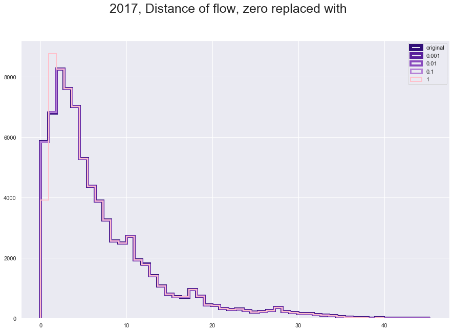
plt.figure(figsize = [15,10])
plt.suptitle("2017, Distance of flow, zero replaced with", fontsize=25)
plt.hist(fl170['great_circle_dist'], histtype='step', linewidth=6 , color = '#310F78', bins = 50)
plt.hist(fl170['dist_adjusted_0001'], histtype='step', linewidth=5 ,color = '#581E9B', bins = 50)
plt.hist(fl170['dist_adjusted_001'], histtype='step', linewidth=4,color = '#894ABD' , bins = 50)
plt.hist(fl170['dist_adjusted_01'], histtype='step',linewidth=3 ,color = '#B581D6', bins = 50)
plt.hist(fl170['dist_adjusted_1'], histtype='step',linewidth=2 ,color = 'pink', bins = 50)
plt.legend(labels=['original','0.001', '0.01', '0.1', '1']);
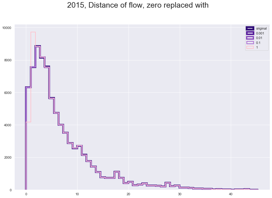
plt.figure(figsize = [15,10])
plt.suptitle("2015, Distance of flow, zero replaced with", fontsize=25)
plt.hist(fl150['great_circle_dist'], histtype='step', linewidth=6 , color = '#310F78', bins = 50)
plt.hist(fl150['dist_adjusted_0001'], histtype='step', linewidth=5 ,color = '#581E9B', bins = 50)
plt.hist(fl150['dist_adjusted_001'], histtype='step', linewidth=4,color = '#894ABD' , bins = 50)
plt.hist(fl150['dist_adjusted_01'], histtype='step',linewidth=3 ,color = '#B581D6', bins = 50)
plt.hist(fl150['dist_adjusted_1'], histtype='step',linewidth=2 ,color = 'pink', bins = 50)
plt.legend(labels=['original','0.001', '0.01', '0.1', '1']);
fl15_sub = fl150
fl16_sub = fl160
fl17_sub = fl170
fl18_sub = fl180
Build the data for the add up
# 0.001
fl15_add = fl15
fl15_add['great_circle_dist_0001'] = fl15_add['great_circle_dist'] + 0.001
fl15_add['NUMBER_OF_PATIENTS_0001'] = fl15_add['NUMBER_OF_PATIENTS'] + 0.001
fl15_add['Density_0001'] = fl15_add['Density'] + 0.001

fl16_add = fl16
fl16_add['great_circle_dist_0001'] = fl16_add['great_circle_dist'] + 0.001
fl16_add['NUMBER_OF_PATIENTS_0001'] = fl16_add['NUMBER_OF_PATIENTS'] + 0.001
fl16_add['Density_0001'] = fl16_add['Density'] + 0.001

fl17_add = fl17
fl17_add['great_circle_dist_0001'] = fl17_add['great_circle_dist'] + 0.001
fl17_add['NUMBER_OF_PATIENTS_0001'] = fl17_add['NUMBER_OF_PATIENTS'] + 0.001
fl17_add['Density_0001'] = fl17_add['Density'] + 0.001

fl18_add = fl18
fl18_add['great_circle_dist_0001'] = fl18_add['great_circle_dist'] + 0.001
fl18_add['NUMBER_OF_PATIENTS_0001'] = fl18_add['NUMBER_OF_PATIENTS'] + 0.001
fl18_add['Density_0001'] = fl18_add['Density'] + 0.001

# 0.01
fl15_add['great_circle_dist_001'] = fl15_add['great_circle_dist'] + 0.01
fl15_add['NUMBER_OF_PATIENTS_001'] = fl15_add['NUMBER_OF_PATIENTS'] + 0.01
fl15_add['Density_001'] = fl15_add['Density'] + 0.01

fl16_add['great_circle_dist_001'] = fl16_add['great_circle_dist'] + 0.01
fl16_add['NUMBER_OF_PATIENTS_001'] = fl16_add['NUMBER_OF_PATIENTS'] + 0.01
fl16_add['Density_001'] = fl16_add['Density'] + 0.01

fl17_add['great_circle_dist_001'] = fl17_add['great_circle_dist'] + 0.01
fl17_add['NUMBER_OF_PATIENTS_001'] = fl17_add['NUMBER_OF_PATIENTS'] + 0.01
fl17_add['Density_001'] = fl17_add['Density'] + 0.01

fl18_add['great_circle_dist_001'] = fl18_add['great_circle_dist'] + 0.01
fl18_add['NUMBER_OF_PATIENTS_001'] = fl18_add['NUMBER_OF_PATIENTS'] + 0.01
fl18_add['Density_001'] = fl18_add['Density'] + 0.01

# 0.1
fl15_add['great_circle_dist_01'] = fl15_add['great_circle_dist'] + 0.1
fl15_add['NUMBER_OF_PATIENTS_01'] = fl15_add['NUMBER_OF_PATIENTS'] + 0.1
fl15_add['Density_01'] = fl15_add['Density'] + 0.1

fl16_add['great_circle_dist_01'] = fl16_add['great_circle_dist'] + 0.1
fl16_add['NUMBER_OF_PATIENTS_01'] = fl16_add['NUMBER_OF_PATIENTS'] + 0.1
fl16_add['Density_01'] = fl16_add['Density'] + 0.1

fl17_add['great_circle_dist_01'] = fl17_add['great_circle_dist'] + 0.1
fl17_add['NUMBER_OF_PATIENTS_01'] = fl17_add['NUMBER_OF_PATIENTS'] + 0.1
fl17_add['Density_01'] = fl17_add['Density'] + 0.1

fl18_add['great_circle_dist_01'] = fl18_add['great_circle_dist'] + 0.1
fl18_add['NUMBER_OF_PATIENTS_01'] = fl18_add['NUMBER_OF_PATIENTS'] + 0.1
fl18_add['Density_01'] = fl18_add['Density'] + 0.1

# 1
fl15_add['great_circle_dist_1'] = fl15_add['great_circle_dist'] + 1
fl15_add['NUMBER_OF_PATIENTS_1'] = fl15_add['NUMBER_OF_PATIENTS'] + 1
fl15_add['Density_1'] = fl15_add['Density'] + 1

fl16_add['great_circle_dist_1'] = fl16_add['great_circle_dist'] + 1
fl16_add['NUMBER_OF_PATIENTS_1'] = fl16_add['NUMBER_OF_PATIENTS'] + 1
fl16_add['Density_1'] = fl16_add['Density'] + 1

fl17_add['great_circle_dist_1'] = fl17_add['great_circle_dist'] + 1
fl17_add['NUMBER_OF_PATIENTS_1'] = fl17_add['NUMBER_OF_PATIENTS'] + 1
fl17_add['Density_1'] = fl17_add['Density'] + 1

fl18_add['great_circle_dist_1'] = fl18_add['great_circle_dist'] + 1
fl18_add['NUMBER_OF_PATIENTS_1'] = fl18_add['NUMBER_OF_PATIENTS'] + 1
fl18_add['Density_1'] = fl18_add['Density'] + 1
plt.figure(figsize = [15,10])
plt.suptitle("2018, Distance of flow, zero replaced with", fontsize=25)
plt.hist(fl18_add['great_circle_dist'], histtype='step', linewidth=6 ,  color = '#310F78', bins = 50)
plt.hist(fl18_add['great_circle_dist_0001'], histtype='step', linewidth=5 ,color = '#581E9B', bins = 50)
plt.hist(fl18_add['great_circle_dist_001'], histtype='step', linewidth=4,color = '#894ABD' , bins = 50)
plt.hist(fl18_add['great_circle_dist_01'], histtype='step',linewidth=3 ,color = '#B581D6', bins = 50)
plt.hist(fl18_add['great_circle_dist_1'], histtype='step',linewidth=2 ,color = 'pink', bins = 50)
plt.legend(labels=['original','0.001', '0.01', '0.1', '1']);

Build the models
# power modes
# 2015
mps531 = Gravity(flows = fl15_sub['N_Items'].astype(int).values, o_vars = fl15_sub['NUMBER_OF_PATIENTS'].values, d_vars = fl15_sub['Density'].values, cost = fl15_sub['dist_adjusted_0001'].values, cost_func = 'pow',   constant=True)
mps521 = Gravity(flows = fl15_sub['N_Items'].astype(int).values, o_vars = fl15_sub['NUMBER_OF_PATIENTS'].values, d_vars = fl15_sub['Density'].values, cost = fl15_sub['dist_adjusted_001'].values, cost_func = 'pow',   constant=True)
mps511 = Gravity(flows = fl15_sub['N_Items'].astype(int).values, o_vars = fl15_sub['NUMBER_OF_PATIENTS'].values, d_vars = fl15_sub['Density'].values, cost = fl15_sub['dist_adjusted_01'].values, cost_func = 'pow',   constant=True)
mps501 = Gravity(flows = fl15_sub['N_Items'].astype(int).values, o_vars = fl15_sub['NUMBER_OF_PATIENTS'].values, d_vars = fl15_sub['Density'].values, cost = fl15_sub['dist_adjusted_1'].values, cost_func = 'pow',   constant=True)
mpa531 = Gravity(flows = fl15_add['N_Items'].astype(int).values, o_vars = fl15_add['NUMBER_OF_PATIENTS_0001'].values, d_vars = fl15_add['Density_0001'].values, cost = fl15_add['great_circle_dist_0001'].values, cost_func = 'pow',   constant=True)
mpa521 = Gravity(flows = fl15_add['N_Items'].astype(int).values, o_vars = fl15_add['NUMBER_OF_PATIENTS_001'].values, d_vars = fl15_add['Density_001'].values, cost = fl15_add['great_circle_dist_001'].values, cost_func = 'pow',   constant=True)
mpa511 = Gravity(flows = fl15_add['N_Items'].astype(int).values, o_vars = fl15_add['NUMBER_OF_PATIENTS_01'].values, d_vars = fl15_add['Density_01'].values, cost = fl15_add['great_circle_dist_01'].values, cost_func = 'pow',   constant=True)
mpa501 = Gravity(flows = fl15_add['N_Items'].astype(int).values, o_vars = fl15_add['NUMBER_OF_PATIENTS_1'].values, d_vars = fl15_add['Density_1'].values, cost = fl15_add['great_circle_dist_1'].values, cost_func = 'pow',   constant=True)
# 2016
mps631 = Gravity(flows = fl16_sub['N_Items'].astype(int).values, o_vars = fl16_sub['NUMBER_OF_PATIENTS'].values, d_vars = fl16_sub['Density'].values, cost = fl16_sub['dist_adjusted_0001'].values, cost_func = 'pow',   constant=True)
mps621 = Gravity(flows = fl16_sub['N_Items'].astype(int).values, o_vars = fl16_sub['NUMBER_OF_PATIENTS'].values, d_vars = fl16_sub['Density'].values, cost = fl16_sub['dist_adjusted_001'].values, cost_func = 'pow',   constant=True)
mps611 = Gravity(flows = fl16_sub['N_Items'].astype(int).values, o_vars = fl16_sub['NUMBER_OF_PATIENTS'].values, d_vars = fl16_sub['Density'].values, cost = fl16_sub['dist_adjusted_01'].values, cost_func = 'pow',   constant=True)
mps601 = Gravity(flows = fl16_sub['N_Items'].astype(int).values, o_vars = fl16_sub['NUMBER_OF_PATIENTS'].values, d_vars = fl16_sub['Density'].values, cost = fl16_sub['dist_adjusted_1'].values, cost_func = 'pow',   constant=True)
mpa631 = Gravity(flows = fl16_add['N_Items'].astype(int).values, o_vars = fl16_add['NUMBER_OF_PATIENTS_0001'].values, d_vars = fl16_add['Density_0001'].values, cost = fl16_add['great_circle_dist_0001'].values, cost_func = 'pow',   constant=True)
mpa621 = Gravity(flows = fl16_add['N_Items'].astype(int).values, o_vars = fl16_add['NUMBER_OF_PATIENTS_001'].values, d_vars = fl16_add['Density_001'].values, cost = fl16_add['great_circle_dist_001'].values, cost_func = 'pow',   constant=True)
mpa611 = Gravity(flows = fl16_add['N_Items'].astype(int).values, o_vars = fl16_add['NUMBER_OF_PATIENTS_01'].values, d_vars = fl16_add['Density_01'].values, cost = fl16_add['great_circle_dist_01'].values, cost_func = 'pow',   constant=True)
mpa601 = Gravity(flows = fl16_add['N_Items'].astype(int).values, o_vars = fl16_add['NUMBER_OF_PATIENTS_1'].values, d_vars = fl16_add['Density_1'].values, cost = fl16_add['great_circle_dist_1'].values, cost_func = 'pow',   constant=True)
# 2017
mps731 = Gravity(flows = fl17_sub['N_Items'].astype(int).values, o_vars = fl17_sub['NUMBER_OF_PATIENTS'].values, d_vars = fl17_sub['Density'].values, cost = fl17_sub['dist_adjusted_0001'].values, cost_func = 'pow',   constant=True)
mps721 = Gravity(flows = fl17_sub['N_Items'].astype(int).values, o_vars = fl17_sub['NUMBER_OF_PATIENTS'].values, d_vars = fl17_sub['Density'].values, cost = fl17_sub['dist_adjusted_001'].values, cost_func = 'pow',   constant=True)
mps711 = Gravity(flows = fl17_sub['N_Items'].astype(int).values, o_vars = fl17_sub['NUMBER_OF_PATIENTS'].values, d_vars = fl17_sub['Density'].values, cost = fl17_sub['dist_adjusted_01'].values, cost_func = 'pow',   constant=True)
mps701 = Gravity(flows = fl17_sub['N_Items'].astype(int).values, o_vars = fl17_sub['NUMBER_OF_PATIENTS'].values, d_vars = fl17_sub['Density'].values, cost = fl17_sub['dist_adjusted_1'].values, cost_func = 'pow',   constant=True)
mpa731 = Gravity(flows = fl17_add['N_Items'].astype(int).values, o_vars = fl17_add['NUMBER_OF_PATIENTS_0001'].values, d_vars = fl17_add['Density_0001'].values, cost = fl17_add['great_circle_dist_0001'].values, cost_func = 'pow',   constant=True)
mpa721 = Gravity(flows = fl17_add['N_Items'].astype(int).values, o_vars = fl17_add['NUMBER_OF_PATIENTS_001'].values, d_vars = fl17_add['Density_001'].values, cost = fl17_add['great_circle_dist_001'].values, cost_func = 'pow',   constant=True)
mpa711 = Gravity(flows = fl17_add['N_Items'].astype(int).values, o_vars = fl17_add['NUMBER_OF_PATIENTS_01'].values, d_vars = fl17_add['Density_01'].values, cost = fl17_add['great_circle_dist_01'].values, cost_func = 'pow',   constant=True)
mpa701 = Gravity(flows = fl17_add['N_Items'].astype(int).values, o_vars = fl17_add['NUMBER_OF_PATIENTS_1'].values, d_vars = fl17_add['Density_1'].values, cost = fl17_add['great_circle_dist_1'].values, cost_func = 'pow',   constant=True)
# 2018
mps831 = Gravity(flows = fl18_sub['N_Items'].astype(int).values, o_vars = fl18_sub['NUMBER_OF_PATIENTS'].values, d_vars = fl18_sub['Density'].values, cost = fl18_sub['dist_adjusted_0001'].values, cost_func = 'pow',   constant=True)
mps821 = Gravity(flows = fl18_sub['N_Items'].astype(int).values, o_vars = fl18_sub['NUMBER_OF_PATIENTS'].values, d_vars = fl18_sub['Density'].values, cost = fl18_sub['dist_adjusted_001'].values, cost_func = 'pow',   constant=True)
mps811 = Gravity(flows = fl18_sub['N_Items'].astype(int).values, o_vars = fl18_sub['NUMBER_OF_PATIENTS'].values, d_vars = fl18_sub['Density'].values, cost = fl18_sub['dist_adjusted_01'].values, cost_func = 'pow',   constant=True)
mps801 = Gravity(flows = fl18_sub['N_Items'].astype(int).values, o_vars = fl18_sub['NUMBER_OF_PATIENTS'].values, d_vars = fl18_sub['Density'].values, cost = fl18_sub['dist_adjusted_1'].values, cost_func = 'pow',   constant=True)
mpa831 = Gravity(flows = fl18_add['N_Items'].astype(int).values, o_vars = fl18_add['NUMBER_OF_PATIENTS_0001'].values, d_vars = fl18_add['Density_0001'].values, cost = fl18_add['great_circle_dist_0001'].values, cost_func = 'pow',   constant=True)
mpa821 = Gravity(flows = fl18_add['N_Items'].astype(int).values, o_vars = fl18_add['NUMBER_OF_PATIENTS_001'].values, d_vars = fl18_add['Density_001'].values, cost = fl18_add['great_circle_dist_001'].values, cost_func = 'pow',   constant=True)
mpa811 = Gravity(flows = fl18_add['N_Items'].astype(int).values, o_vars = fl18_add['NUMBER_OF_PATIENTS_01'].values, d_vars = fl18_add['Density_01'].values, cost = fl18_add['great_circle_dist_01'].values, cost_func = 'pow',   constant=True)
mpa801 = Gravity(flows = fl18_add['N_Items'].astype(int).values, o_vars = fl18_add['NUMBER_OF_PATIENTS_1'].values, d_vars = fl18_add['Density_1'].values, cost = fl18_add['great_circle_dist_1'].values, cost_func = 'pow',   constant=True)
# exponential models
# base, no change
base5 = Gravity(flows = fl15_sub['N_Items'].astype(int).values, o_vars = fl15_sub['NUMBER_OF_PATIENTS'].values, d_vars = fl15_sub['Density'].values, cost = fl15_sub['great_circle_dist'].values, cost_func = 'exp',   constant=True)
base6 = Gravity(flows = fl16_sub['N_Items'].astype(int).values, o_vars = fl16_sub['NUMBER_OF_PATIENTS'].values, d_vars = fl16_sub['Density'].values, cost = fl16_sub['great_circle_dist'].values, cost_func = 'exp',   constant=True)
base7 = Gravity(flows = fl17_sub['N_Items'].astype(int).values, o_vars = fl17_sub['NUMBER_OF_PATIENTS'].values, d_vars = fl17_sub['Density'].values, cost = fl17_sub['great_circle_dist'].values, cost_func = 'exp',   constant=True)
base8 = Gravity(flows = fl18_sub['N_Items'].astype(int).values, o_vars = fl18_sub['NUMBER_OF_PATIENTS'].values, d_vars = fl18_sub['Density'].values, cost = fl18_sub['great_circle_dist'].values, cost_func = 'exp',   constant=True)
# 2015
mes531 = Gravity(flows = fl15_sub['N_Items'].astype(int).values, o_vars = fl15_sub['NUMBER_OF_PATIENTS'].values, d_vars = fl15_sub['Density'].values, cost = fl15_sub['dist_adjusted_0001'].values, cost_func = 'exp',   constant=True)
mes521 = Gravity(flows = fl15_sub['N_Items'].astype(int).values, o_vars = fl15_sub['NUMBER_OF_PATIENTS'].values, d_vars = fl15_sub['Density'].values, cost = fl15_sub['dist_adjusted_001'].values, cost_func = 'exp',   constant=True)
mes511 = Gravity(flows = fl15_sub['N_Items'].astype(int).values, o_vars = fl15_sub['NUMBER_OF_PATIENTS'].values, d_vars = fl15_sub['Density'].values, cost = fl15_sub['dist_adjusted_01'].values, cost_func = 'exp',   constant=True)
mes501 = Gravity(flows = fl15_sub['N_Items'].astype(int).values, o_vars = fl15_sub['NUMBER_OF_PATIENTS'].values, d_vars = fl15_sub['Density'].values, cost = fl15_sub['dist_adjusted_1'].values, cost_func = 'exp',   constant=True)
mea531 = Gravity(flows = fl15_add['N_Items'].astype(int).values, o_vars = fl15_add['NUMBER_OF_PATIENTS_0001'].values, d_vars = fl15_add['Density_0001'].values, cost = fl15_add['great_circle_dist_0001'].values, cost_func = 'exp',   constant=True)
mea521 = Gravity(flows = fl15_add['N_Items'].astype(int).values, o_vars = fl15_add['NUMBER_OF_PATIENTS_001'].values, d_vars = fl15_add['Density_001'].values, cost = fl15_add['great_circle_dist_001'].values, cost_func = 'exp',   constant=True)
mea511 = Gravity(flows = fl15_add['N_Items'].astype(int).values, o_vars = fl15_add['NUMBER_OF_PATIENTS_01'].values, d_vars = fl15_add['Density_01'].values, cost = fl15_add['great_circle_dist_01'].values, cost_func = 'exp',   constant=True)
mea501 = Gravity(flows = fl15_add['N_Items'].astype(int).values, o_vars = fl15_add['NUMBER_OF_PATIENTS_1'].values, d_vars = fl15_add['Density_1'].values, cost = fl15_add['great_circle_dist_1'].values, cost_func = 'exp',   constant=True)
# 2016
mes631 = Gravity(flows = fl16_sub['N_Items'].astype(int).values, o_vars = fl16_sub['NUMBER_OF_PATIENTS'].values, d_vars = fl16_sub['Density'].values, cost = fl16_sub['dist_adjusted_0001'].values, cost_func = 'exp',   constant=True)
mes621 = Gravity(flows = fl16_sub['N_Items'].astype(int).values, o_vars = fl16_sub['NUMBER_OF_PATIENTS'].values, d_vars = fl16_sub['Density'].values, cost = fl16_sub['dist_adjusted_001'].values, cost_func = 'exp',   constant=True)
mes611 = Gravity(flows = fl16_sub['N_Items'].astype(int).values, o_vars = fl16_sub['NUMBER_OF_PATIENTS'].values, d_vars = fl16_sub['Density'].values, cost = fl16_sub['dist_adjusted_01'].values, cost_func = 'exp',   constant=True)
mes601 = Gravity(flows = fl16_sub['N_Items'].astype(int).values, o_vars = fl16_sub['NUMBER_OF_PATIENTS'].values, d_vars = fl16_sub['Density'].values, cost = fl16_sub['dist_adjusted_1'].values, cost_func = 'exp',   constant=True)
mea631 = Gravity(flows = fl16_add['N_Items'].astype(int).values, o_vars = fl16_add['NUMBER_OF_PATIENTS_0001'].values, d_vars = fl16_add['Density_0001'].values, cost = fl16_add['great_circle_dist_0001'].values, cost_func = 'exp',   constant=True)
mea621 = Gravity(flows = fl16_add['N_Items'].astype(int).values, o_vars = fl16_add['NUMBER_OF_PATIENTS_001'].values, d_vars = fl16_add['Density_001'].values, cost = fl16_add['great_circle_dist_001'].values, cost_func = 'exp',   constant=True)
mea611 = Gravity(flows = fl16_add['N_Items'].astype(int).values, o_vars = fl16_add['NUMBER_OF_PATIENTS_01'].values, d_vars = fl16_add['Density_01'].values, cost = fl16_add['great_circle_dist_01'].values, cost_func = 'exp',   constant=True)
mea601 = Gravity(flows = fl16_add['N_Items'].astype(int).values, o_vars = fl16_add['NUMBER_OF_PATIENTS_1'].values, d_vars = fl16_add['Density_1'].values, cost = fl16_add['great_circle_dist_1'].values, cost_func = 'exp',   constant=True)
# 2017
mes731 = Gravity(flows = fl17_sub['N_Items'].astype(int).values, o_vars = fl17_sub['NUMBER_OF_PATIENTS'].values, d_vars = fl17_sub['Density'].values, cost = fl17_sub['dist_adjusted_0001'].values, cost_func = 'exp',   constant=True)
mes721 = Gravity(flows = fl17_sub['N_Items'].astype(int).values, o_vars = fl17_sub['NUMBER_OF_PATIENTS'].values, d_vars = fl17_sub['Density'].values, cost = fl17_sub['dist_adjusted_001'].values, cost_func = 'exp',   constant=True)
mes711 = Gravity(flows = fl17_sub['N_Items'].astype(int).values, o_vars = fl17_sub['NUMBER_OF_PATIENTS'].values, d_vars = fl17_sub['Density'].values, cost = fl17_sub['dist_adjusted_01'].values, cost_func = 'exp',   constant=True)
mes701 = Gravity(flows = fl17_sub['N_Items'].astype(int).values, o_vars = fl17_sub['NUMBER_OF_PATIENTS'].values, d_vars = fl17_sub['Density'].values, cost = fl17_sub['dist_adjusted_1'].values, cost_func = 'exp',   constant=True)
mea731 = Gravity(flows = fl17_add['N_Items'].astype(int).values, o_vars = fl17_add['NUMBER_OF_PATIENTS_0001'].values, d_vars = fl17_add['Density_0001'].values, cost = fl17_add['great_circle_dist_0001'].values, cost_func = 'exp',   constant=True)
mea721 = Gravity(flows = fl17_add['N_Items'].astype(int).values, o_vars = fl17_add['NUMBER_OF_PATIENTS_001'].values, d_vars = fl17_add['Density_001'].values, cost = fl17_add['great_circle_dist_001'].values, cost_func = 'exp',   constant=True)
mea711 = Gravity(flows = fl17_add['N_Items'].astype(int).values, o_vars = fl17_add['NUMBER_OF_PATIENTS_01'].values, d_vars = fl17_add['Density_01'].values, cost = fl17_add['great_circle_dist_01'].values, cost_func = 'exp',   constant=True)
mea701 = Gravity(flows = fl17_add['N_Items'].astype(int).values, o_vars = fl17_add['NUMBER_OF_PATIENTS_1'].values, d_vars = fl17_add['Density_1'].values, cost = fl17_add['great_circle_dist_1'].values, cost_func = 'exp',   constant=True)
# 2018
mes831 = Gravity(flows = fl18_sub['N_Items'].astype(int).values, o_vars = fl18_sub['NUMBER_OF_PATIENTS'].values, d_vars = fl18_sub['Density'].values, cost = fl18_sub['dist_adjusted_0001'].values, cost_func = 'exp',   constant=True)
mes821 = Gravity(flows = fl18_sub['N_Items'].astype(int).values, o_vars = fl18_sub['NUMBER_OF_PATIENTS'].values, d_vars = fl18_sub['Density'].values, cost = fl18_sub['dist_adjusted_001'].values, cost_func = 'exp',   constant=True)
mes811 = Gravity(flows = fl18_sub['N_Items'].astype(int).values, o_vars = fl18_sub['NUMBER_OF_PATIENTS'].values, d_vars = fl18_sub['Density'].values, cost = fl18_sub['dist_adjusted_01'].values, cost_func = 'exp',   constant=True)
mes801 = Gravity(flows = fl18_sub['N_Items'].astype(int).values, o_vars = fl18_sub['NUMBER_OF_PATIENTS'].values, d_vars = fl18_sub['Density'].values, cost = fl18_sub['dist_adjusted_1'].values, cost_func = 'exp',   constant=True)
mea831 = Gravity(flows = fl18_add['N_Items'].astype(int).values, o_vars = fl18_add['NUMBER_OF_PATIENTS_0001'].values, d_vars = fl18_add['Density_0001'].values, cost = fl18_add['great_circle_dist_0001'].values, cost_func = 'exp',   constant=True)
mea821 = Gravity(flows = fl18_add['N_Items'].astype(int).values, o_vars = fl18_add['NUMBER_OF_PATIENTS_001'].values, d_vars = fl18_add['Density_001'].values, cost = fl18_add['great_circle_dist_001'].values, cost_func = 'exp',   constant=True)
mea811 = Gravity(flows = fl18_add['N_Items'].astype(int).values, o_vars = fl18_add['NUMBER_OF_PATIENTS_01'].values, d_vars = fl18_add['Density_01'].values, cost = fl18_add['great_circle_dist_01'].values, cost_func = 'exp',   constant=True)
mea801 = Gravity(flows = fl18_add['N_Items'].astype(int).values, o_vars = fl18_add['NUMBER_OF_PATIENTS_1'].values, d_vars = fl18_add['Density_1'].values, cost = fl18_add['great_circle_dist_1'].values, cost_func = 'exp',   constant=True)
R215, R216, R217, R218 = [], [], [], []
model_nameP = ['gravity_power_sub_0.001', 'gravity_power_sub_0.01',  'gravity_power_sub_0.1','gravity_power_sub_1', 'gravity_power_add_0.001', 'gravity_power_add_0.01', 'gravity_power_add_0.1', 'gravity_power_add_1']
col_namesP = ['R2_2015', 'R2_2016', 'R2_2017', 'R2_2018']
models15 = [mps531, mps521, mps511, mps501, mpa531,mpa521,mpa511,mpa501]
models16 = [mps631, mps621, mps611, mps601, mpa631,mpa621,mpa611,mpa601]
models17 = [mps731, mps721, mps711, mps701, mpa731,mpa721,mpa711,mpa701]
models18 = [mps831, mps821, mps811, mps801, mpa831,mpa821,mpa811,mpa801]

for model in models15:
    R215.append(model.pseudoR2)
for model in models16:
    R216.append(model.pseudoR2)
for model in models17:
    R217.append(model.pseudoR2)
for model in models18:
    R218.append(model.pseudoR2)

colsP = {'model_name': model_nameP,'R2_2015': R215, 'R2_2016': R216,'R2_2017': R217,'R2_2018': R218}

dataP = pd.DataFrame(colsP).set_index('model_name')
R215, R216, R217, R218 = [], [], [], []
model_nameE = ['base_exponential','gravity_exponent_sub_0.001', 'gravity_exponent_sub_0.01',  'gravity_exponent_sub_0.1','gravity_exponent_sub_1', 'gravity_exponent_add_0.001', 'gravity_exponent_add_0.01', 'gravity_exponent_add_0.1', 'gravity_exponent_add_1']
col_namesE = ['R2_2015', 'R2_2016', 'R2_2017', 'R2_2018']
models15 = [base5, mes531, mes521, mes511, mes501, mea531,mea521,mea511,mea501]
models16 = [base6, mes631, mes621, mes611, mes601, mea631,mea621,mea611,mea601]
models17 = [base7, mes731, mes721, mes711, mes701, mea731,mea721,mea711,mea701]
models18 = [base8, mes831, mes821, mes811, mes801, mea831,mea821,mea811,mea801]

for model in models15:
    R215.append(model.pseudoR2)
for model in models16:
    R216.append(model.pseudoR2)
for model in models17:
    R217.append(model.pseudoR2)
for model in models18:
    R218.append(model.pseudoR2)

colsE = {'model_name': model_nameE,'R2_2015': R215, 'R2_2016': R216,'R2_2017': R217,'R2_2018': R218}

dataE = pd.DataFrame(colsE).set_index('model_name')
dataE[col_namesE]
| R2_2015 | R2_2016 | R2_2017 | R2_2018 | |
|---|---|---|---|---|
| model_name | ||||
| base_exponential | 0.577145 | 0.572300 | 0.559345 | 0.557001 |
| gravity_exponent_sub_0.001 | 0.577135 | 0.572288 | 0.559332 | 0.556991 |
| gravity_exponent_sub_0.01 | 0.577047 | 0.572181 | 0.559213 | 0.556892 |
| gravity_exponent_sub_0.1 | 0.575993 | 0.570945 | 0.557879 | 0.555773 |
| gravity_exponent_sub_1 | 0.546718 | 0.540835 | 0.529192 | 0.529886 |
| gravity_exponent_add_0.001 | 0.577149 | 0.572303 | 0.559348 | 0.557006 |
| gravity_exponent_add_0.01 | 0.577181 | 0.572333 | 0.559381 | 0.557043 |
| gravity_exponent_add_0.1 | 0.577483 | 0.572611 | 0.559688 | 0.557389 |
| gravity_exponent_add_1 | 0.579162 | 0.574184 | 0.561462 | 0.559391 |
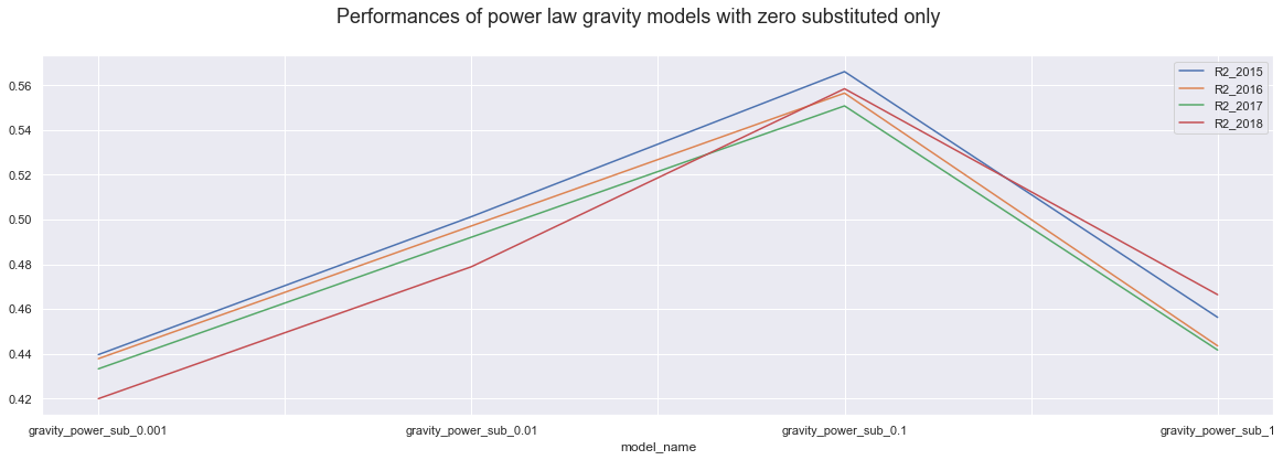
dataP[col_namesP]
| R2_2015 | R2_2016 | R2_2017 | R2_2018 | |
|---|---|---|---|---|
| model_name | ||||
| gravity_power_sub_0.001 | 0.439593 | 0.437777 | 0.433232 | 0.419891 |
| gravity_power_sub_0.01 | 0.501261 | 0.497098 | 0.492077 | 0.478877 |
| gravity_power_sub_0.1 | 0.566077 | 0.556465 | 0.550752 | 0.558417 |
| gravity_power_sub_1 | 0.456260 | 0.443518 | 0.441651 | 0.466390 |
| gravity_power_add_0.001 | 0.439037 | 0.437308 | 0.432843 | 0.419657 |
| gravity_power_add_0.01 | 0.498087 | 0.494550 | 0.489984 | 0.476431 |
| gravity_power_add_0.1 | 0.578871 | 0.572455 | 0.567675 | 0.555453 |
| gravity_power_add_1 | 0.632234 | 0.623348 | 0.617584 | 0.611254 |
Conlusion
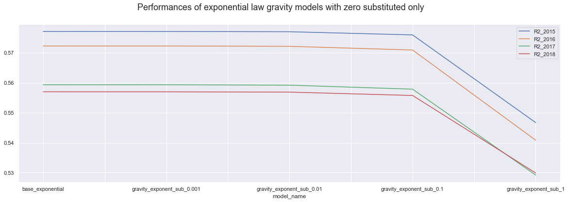
dataE.iloc[0:5,].plot()
plt.suptitle("Performances of exponential law gravity models with zero substituted only", fontsize=18);
dataP.iloc[0:4,].plot()
plt.suptitle("Performances of power law gravity models with zero substituted only", fontsize=18);
dataE.iloc[5:9,].plot()
plt.suptitle("Performances of exponential law gravity models with added values to independent vars", fontsize=18);
dataP.iloc[4:8,].plot()
plt.suptitle("Performances of power law gravity models with added values to independent vars", fontsize=18);
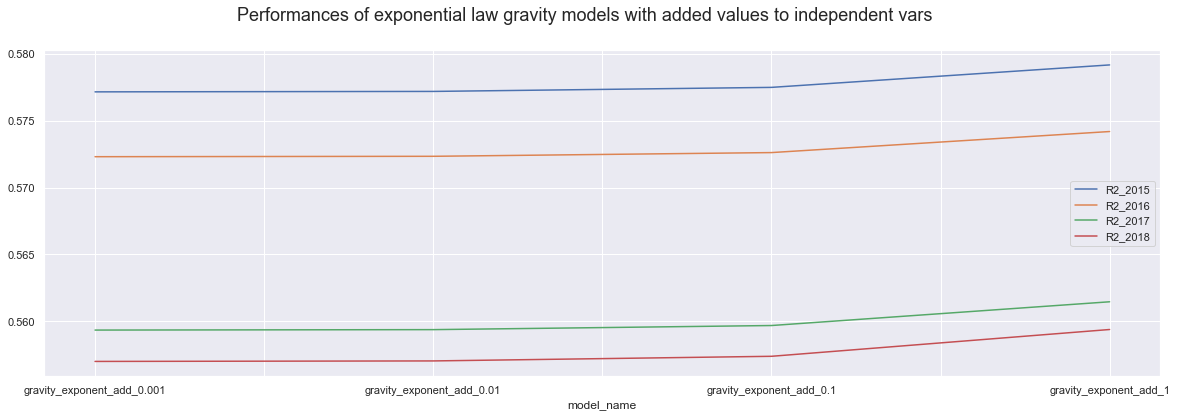
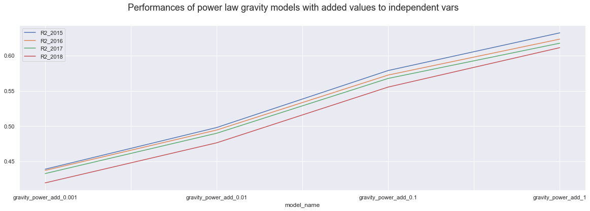
Firstly, we know that the higher value we add up or substitute, the more drastic the change is and the less trust we have into the model accuracy. It is interesting though That using power law models, adding 1 to all variables actually results in the best model of all, over 60%.
Secondly, In all case, power law models show bigger accuracy differences every step we use higher value. On the other hand exponential law models seems to be more stable for the values belw the one, and only show visible difference when we use value of 1.
Thirdly, the power law models perform similarly for all years, but the exponential law models perform much better in teh 2015 and 2016 then in 217 and 2018. However, the difference is less truth when we only substitute the zero and more drastic when we are adding up values.
Why is it so?
- Could it be the Number of patient's variable that is dodgy for the last two years?
- Something else?
Which model to choose
From this, I am Inclining to exponential law model, as they seem to be more stable across little changes. It also can be more advantegous im the future work;
The advantages of the exponential gravity model are as below: first, it is independent of dimension; second, its underlying rationale is clear because it is derivable from the principle of entropy maximization (Chen, 2015)
Then, the base exponential model is actually working without any changes and results in same accuracy as the little changes. So Is there any reason for not to use the base exponential model?
cost function for the power law model in SpInt
$$np.log$$
cost function for the exponential law model in SpInt
$$\lambda x: x * 1.0$$
## If best model is the base exponential (base8,7,6,5) the we can test what the same model does with th ecomplete data

file = './../../data/NHS/working/year_data_flow/complete_flow_2017.csv'
comp_fl17 = pd.read_csv(file, index_col=None)
plt.figure(figsize = [15,10])
plt.suptitle("Number of prescriptions on a flow in 2017", fontsize=25)
plt.hist(comp_fl17['N_Items'], histtype='step', linewidth=6, color = '#310F78')
plt.hist(fl17['N_Items'], histtype='step', linewidth=4, color = '#B581D6')
plt.legend(labels=['complete data with 0', 'incomplete as published']);
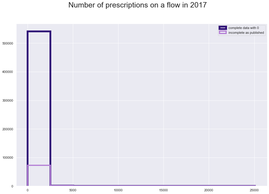
comp_fl17['N_Items'].value_counts()
0.0       469076
1.0        15262
2.0         8029
3.0         5120
4.0         3601
           ...
3911.0         1
6502.0         1
3905.0         1
3901.0         1
2216.0         1
Name: N_Items, Length: 3921, dtype: int64
print( str(round((469076/len(comp_fl17))*100,2)) + '% of the complete data is 0')
86.27% of the complete data is 0
comp_fl17['dist_adjusted_0001'] = comp_fl17['great_circle_dist'].mask(comp_fl17['great_circle_dist'] == 0, 0.001)
comp_base7 = Gravity(flows = comp_fl17['N_Items'].astype(int).values, o_vars = comp_fl17['NUMBER_OF_PATIENTS'].values, d_vars = comp_fl17['Density'].values, cost = comp_fl17['great_circle_dist'].values, cost_func = 'exp',   constant=True)
comp_base7_eucd = Gravity(flows = comp_fl17['N_Items'].astype(int).values, o_vars = comp_fl17['NUMBER_OF_PATIENTS'].values, d_vars = comp_fl17['Density'].values, cost = comp_fl17['Euc_distance'].values, cost_func = 'exp',   constant=True)
comp_base7_pow = Gravity(flows = comp_fl17['N_Items'].astype(int).values, o_vars = comp_fl17['NUMBER_OF_PATIENTS'].values, d_vars = comp_fl17['Density'].values, cost = comp_fl17['dist_adjusted_0001'].values, cost_func = 'pow',   constant=True)
print('complete data, great circle distance, pseudo R2 ' + str(round(comp_base7.pseudoR2,2)))
print('complete data, euclidian distance, pseudo R2 ' + str(round(comp_base7_eucd.pseudoR2,2)))
print('complete data, power law, adjusted 0.001, pseudo R2 ' + str(round(comp_base7_pow.pseudoR2,2)))
complete data, great circle distance, pseudo R2 0.67
complete data, euclidian distance, pseudo R2 0.65
complete data, power law, adjusted 0.001, pseudo R2 0.48
print('published data, great circle distance, pseudo R2 ' + str(round(base7.pseudoR2,2)))
published data, great circle distance, pseudo R2 0.56
from scipy import sparse as sp
import numpy as np
from collections import defaultdict
from functools import partial
from itertools import count

def CPC(model):
    """
    Common part of commuters based on Sorensen index
    Lenormand et al. 2012
    """
    y = model.y
    try:
        yhat = model.yhat.resahpe((-1, 1))
    except BaseException:
        yhat = model.mu((-1, 1))
    N = model.n
    YYhat = np.hstack([y, yhat])
    NCC = np.sum(np.min(YYhat, axis=1))
    NCY = np.sum(Y)
    NCYhat = np.sum(yhat)
    return (N * NCC) / (NCY + NCYhat)


def sorensen(model):
    """
    Sorensen similarity index
    For use on spatial interaction models; N = sample size
    rather than N = number of locations and normalized by N instead of N**2
    """
    try:
        y = model.y.reshape((-1, 1))
    except BaseException:
        y = model.f.reshape((-1, 1))
    try:
        yhat = model.yhat.reshape((-1, 1))
    except BaseException:
        yhat = model.mu.reshape((-1, 1))
    N = model.n
    YYhat = np.hstack([y, yhat])
    num = 2.0 * np.min(YYhat, axis=1)
    den = yhat + y
    return (1.0 / N) * (np.sum(num.reshape((-1, 1)) / den.reshape((-1, 1))))
CPC(base7)
# but the SpInt has already sorensen index in it
base7.SSI
0.3182449860984687
comp_base7.SSI
0.04548680791330862
base7.n
74668