Calculating Walking distance in Python. Networkx vs Pandana.
There is no need for GPU when Pandana is at least 1000 times faster.

Introduction
Let's say you have spatial point data and you want to calculate walking distances between all combination of the points. For example, you have data of local bars and you want to find out all the walking distances between them, so you can include them in your regression model (or anything else), for example as a variable that defines how accessible two pubs are to each other.
This post will show you how you can do that in python using
- osmnx package to generate OSM road network
- networkx package to find the nearest point on that network and calulate the walking distance between them
- pandana package to make this significantly faster!
Data
Availiable here
Background
You might need some essential information that will help you to understand what we are doing here. Feel free to skip this part and go straight to the code.
What is the walking distance?
It's exactly what it says. Walking distance from one place to another. In other words, how far is the place from where I stand along the walking path. This information is crucial for estimating how long is it going to take me to go there, how much effort or money will this cost me. Those are all variables that contribute to estimations of accessibility, connectivity, mobility or others.
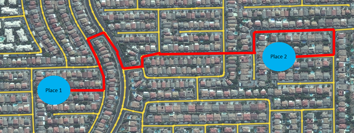
Estimating the walking distance.
The distance between two places/nodes is then the sum of the weights/lengths of all the paths/roads/edges that connects them.
This can be also referred to as the Shortest Path Problem, in which we are looking for the most efficient paths between nodes.
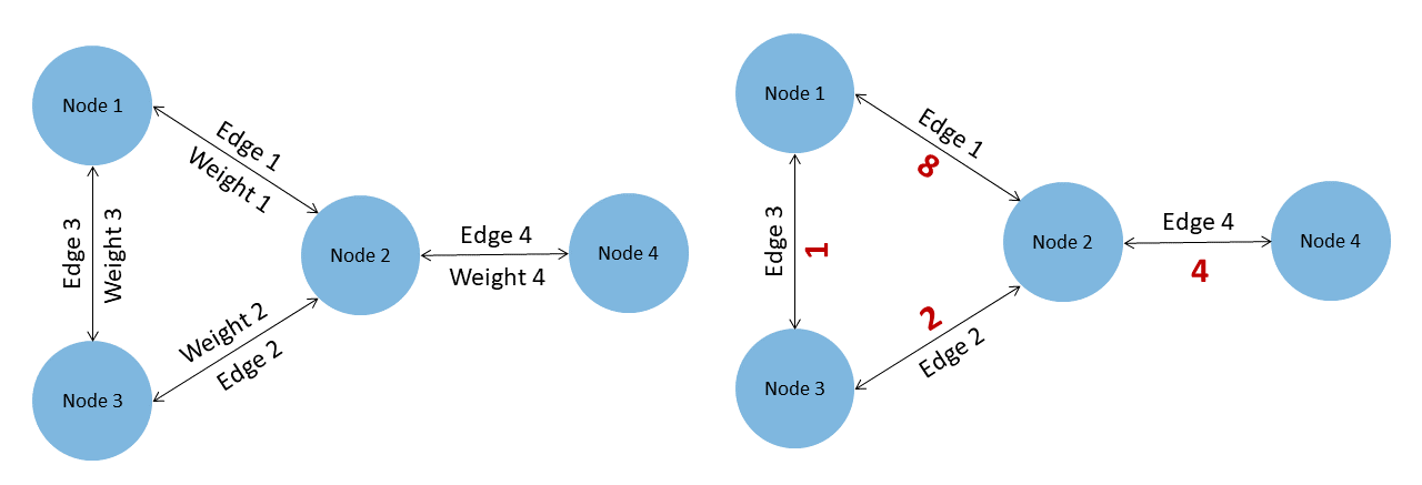
In this example, the shortest path between Node 1 and Node 2 is the $$SUM(Weight 3, Weight 2, Weight 4)$$. So if the weights represent a number of minutes (how long it takes to walk that path) then we would walk for 7 minutes. $$ 1+2+4=7$$
If would choose to go the other way, which is seemingly shorter, $$SUM(Weight 1, Weight 4)$$ $$8+4=12$$ We would walk for 12 minutes. Therefore the first option is the most efficient one.
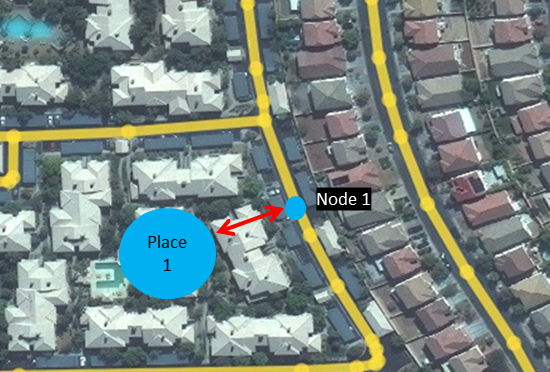
Find the Nearest Neighbour
In any scenarios where the places you want to use for your analysis are not directly placed on the road or path, we need to connect the place to the network. We do this by finding the Nearest neighbouring node on the graph/network to the specific place. Both packages (networkx and pandana) have their own functions that can be used for these purposes.
Load the packages
import pandas as pd
import numpy as np
import geopandas as gpd
import matplotlib.pyplot as plt
import osmnx as ox # install osmnx first, it will download appropriate version of networkx
import networkx as nx
from pyproj import CRS
import itertools

import pandana
print(pandana.__version__)
# define coordinates if you need them
wgs84 = CRS(4326)
bng = CRS(27700)
print(wgs84)
epsg:4326
Load the point data and create flows
pois = gpd.read_file("./points.geojson")
#pois.crs # check the CRS
pois.head()
| ID_code | X | Y | geometry | |
|---|---|---|---|---|
| 0 | A91120 | -2.559063 | 51.502830 | POINT (-2.55906 51.50283) |
| 1 | A99931 | -2.596140 | 51.459182 | POINT (-2.59614 51.45918) |
| 2 | A99986 | -2.538833 | 51.483143 | POINT (-2.53883 51.48314) |
| 3 | L81002 | -2.930352 | 51.360207 | POINT (-2.93035 51.36021) |
| 4 | L81004 | -2.767317 | 51.482805 | POINT (-2.76732 51.48281) |
# tale first 5 points and find all possinle combinations
pois = pois.iloc[0:6,:]

# create a list of all the ID's
p_li = list(pois['ID_code'].unique())

# get all unique combinations of all the origins and destinations
flows = pd.DataFrame(list(itertools.product(p_li,p_li))).rename(columns = {0:'origin',1:'destination'})

flows.info()
<class 'pandas.core.frame.DataFrame'>
RangeIndex: 36 entries, 0 to 35
Data columns (total 2 columns):
 #   Column       Non-Null Count  Dtype
---  ------       --------------  -----
 0   origin       36 non-null     object
 1   destination  36 non-null     object
dtypes: object(2)
memory usage: 704.0+ bytes
Using Networkx
Load Graph
The osmnx package has very useful function ‘graph_from_bbox’ which loads the osm roads graph quite quickly. Here I am loading walking paths for whola area of Avon where my points are located, which is quite a big area so expect this to take few minutes.
# create bounding box for our data
bbox = [51.623985, 51.291124,  -2.272797, -3.029480]

# generate graph based on the bounding box
avon = ox.graph_from_bbox(bbox[0], bbox[1], bbox[2], bbox[3],
                               retain_all=False,
                               truncate_by_edge=True,
                               simplify=False,
                               network_type='walk')
# get the nodes and the edges into geopandas
nodes, edges = ox.graph_to_gdfs(avon, nodes=True, edges=True)
Find the nearest node to each point with osmnx.get_nearest_node()
# define function for the nearest neighbour
def nearest_node(a,b):
    nearest_node,dist=ox.get_nearest_node(avon, (a,b), return_dist=True, method = 'euclidean')
    return nearest_node
# apply the function
pois['NX_node'] = np.vectorize(nearest_node)(pois['Y'],pois['X'])
pois.head()
| ID_code | X | Y | geometry | NX_node | |
|---|---|---|---|---|---|
| 0 | A91120 | -2.559063 | 51.502830 | POINT (-2.55906 51.50283) | 2914306154 |
| 1 | A99931 | -2.596140 | 51.459182 | POINT (-2.59614 51.45918) | 1859320333 |
| 2 | A99986 | -2.538833 | 51.483143 | POINT (-2.53883 51.48314) | 2094196650 |
| 3 | L81002 | -2.930352 | 51.360207 | POINT (-2.93035 51.36021) | 317399984 |
| 4 | L81004 | -2.767317 | 51.482805 | POINT (-2.76732 51.48281) | 2488740793 |
# create list of the node id's and check if they exist and if they are on the right place
nodelist = list(pois['NX_node'].unique())

nodes[nodes.index.isin(nodelist)]
| y | x | street_count | highway | ref | geometry | |
|---|---|---|---|---|---|---|
| osmid | ||||||
| 317399984 | 51.360246 | -2.930589 | 2 | NaN | NaN | POINT (-2.93059 51.36025) |
| 1859320333 | 51.459442 | -2.596420 | 2 | NaN | NaN | POINT (-2.59642 51.45944) |
| 2094196650 | 51.482695 | -2.538694 | 2 | NaN | NaN | POINT (-2.53869 51.48270) |
| 2424544775 | 51.413646 | -2.571651 | 2 | NaN | NaN | POINT (-2.57165 51.41365) |
| 2488740793 | 51.483134 | -2.767173 | 2 | NaN | NaN | POINT (-2.76717 51.48313) |
| 2914306154 | 51.502744 | -2.558880 | 1 | NaN | NaN | POINT (-2.55888 51.50274) |
# get the node id's to flow data
# create two seperate data the target origins and target destinations with the XY coordinates
flows_full = flows.merge(pois.loc[:, pois.columns != 'geometry'], left_on = 'origin', right_on = 'ID_code', how = 'left')

# lets just rename everything for the sake of clarity
flows_full = flows_full.merge(pois.loc[:, pois.columns != 'geometry'], left_on = 'destination', right_on = 'ID_code', how = 'left').rename(columns = {'NX_node_x':'node_o','NX_node_y':'node_d', 'X_x':'X_o','Y_x':'Y_o', 'X_y':'X_d','Y_y':'Y_d', 'ID_code_x':'ID_code_o', 'ID_code_y':'ID_code_d'})

flows_full.head()
| origin | destination | ID_code_o | X_o | Y_o | node_o | ID_code_d | X_d | Y_d | node_d | |
|---|---|---|---|---|---|---|---|---|---|---|
| 0 | A91120 | A91120 | A91120 | -2.559063 | 51.50283 | 2914306154 | A91120 | -2.559063 | 51.502830 | 2914306154 |
| 1 | A91120 | A99931 | A91120 | -2.559063 | 51.50283 | 2914306154 | A99931 | -2.596140 | 51.459182 | 1859320333 |
| 2 | A91120 | A99986 | A91120 | -2.559063 | 51.50283 | 2914306154 | A99986 | -2.538833 | 51.483143 | 2094196650 |
| 3 | A91120 | L81002 | A91120 | -2.559063 | 51.50283 | 2914306154 | L81002 | -2.930352 | 51.360207 | 317399984 |
| 4 | A91120 | L81004 | A91120 | -2.559063 | 51.50283 | 2914306154 | L81004 | -2.767317 | 51.482805 | 2488740793 |
Check that the nodes are on the corect place
# check that the nodes are close to the points
plt.figure( figsize=(10,10))
fig = plt.plot()
ax = plt.axes()

nodes[nodes.index.isin(nodelist)].plot(ax=ax, markersize = 60, color="b" )
pois.plot(ax=ax, markersize = 20, color="r")

plt.show();
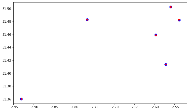
Looks fine to me
Apply the networkx.shortest_path_length
# define a function that calculates shortest path between the nodes on graph
def path_length(row):
    return nx.shortest_path_length(avon, row['node_o'], row['node_d'], weight='length')

# apply the function to our OD data
%timeit flows_full['path_length'] = flows_full.apply(path_length, axis=1)
26.8 s ± 1.58 s per loop (mean ± std. dev. of 7 runs, 1 loop each)
# This is approximately
print(str(round((26.8*(7*1))/60,2)) + ' minutes')
3.13 minutes
flows_full.head()
| origin | destination | ID_code_o | X_o | Y_o | node_o | ID_code_d | X_d | Y_d | node_d | path_length | |
|---|---|---|---|---|---|---|---|---|---|---|---|
| 0 | A91120 | A91120 | A91120 | -2.559063 | 51.50283 | 2914306154 | A91120 | -2.559063 | 51.502830 | 2914306154 | 0.000 |
| 1 | A91120 | A99931 | A91120 | -2.559063 | 51.50283 | 2914306154 | A99931 | -2.596140 | 51.459182 | 1859320333 | 6960.514 |
| 2 | A91120 | A99986 | A91120 | -2.559063 | 51.50283 | 2914306154 | A99986 | -2.538833 | 51.483143 | 2094196650 | 4333.457 |
| 3 | A91120 | L81002 | A91120 | -2.559063 | 51.50283 | 2914306154 | L81002 | -2.930352 | 51.360207 | 317399984 | 36334.316 |
| 4 | A91120 | L81004 | A91120 | -2.559063 | 51.50283 | 2914306154 | L81004 | -2.767317 | 51.482805 | 2488740793 | 19754.732 |
Using Pandana
Load the graph
Listen, I have tried to use the osm loader inside the pandana, but it took ages. after 2 hours of loading, I decided it will be easier to get the previously loaded osm graph with osmnx and use that as a base for the pandana graph. You can just simply use the geodataframes of nodes and flows for the base of your graph.
# reset index so our origins and destinations are not in idnex
edges = edges.reset_index()

# create network with pandana
avon_pan = pandana.Network(nodes['x'], nodes['y'],
                          edges['u'], edges['v'], edges[['length']])
Find the nearest nodes to our points in pandana graph
# we are going to define the origins and destinations separately as alist
# get_node_ids uses kdtree writen in c++, google it its like a magic

origin_nodes = avon_pan.get_node_ids(flows_full.X_o, flows_full.Y_o).values


dests_nodes = avon_pan.get_node_ids(flows_full.X_d, flows_full.Y_d).values
flows_full.head()
| origin | destination | ID_code_o | X_o | Y_o | node_o | ID_code_d | X_d | Y_d | node_d | path_length | |
|---|---|---|---|---|---|---|---|---|---|---|---|
| 0 | A91120 | A91120 | A91120 | -2.559063 | 51.50283 | 2914306154 | A91120 | -2.559063 | 51.502830 | 2914306154 | 0.000 |
| 1 | A91120 | A99931 | A91120 | -2.559063 | 51.50283 | 2914306154 | A99931 | -2.596140 | 51.459182 | 1859320333 | 6960.514 |
| 2 | A91120 | A99986 | A91120 | -2.559063 | 51.50283 | 2914306154 | A99986 | -2.538833 | 51.483143 | 2094196650 | 4333.457 |
| 3 | A91120 | L81002 | A91120 | -2.559063 | 51.50283 | 2914306154 | L81002 | -2.930352 | 51.360207 | 317399984 | 36334.316 |
| 4 | A91120 | L81004 | A91120 | -2.559063 | 51.50283 | 2914306154 | L81004 | -2.767317 | 51.482805 | 2488740793 | 19754.732 |
Calculate distances using pandana ‘shortest_path_lengths’
%%time
flows_full['distances'] = pd.Series(avon_pan.shortest_path_lengths(origin_nodes, dests_nodes))
Wall time: 144 ms
# How much faster is this from networkx
(((3.13*60)*1000))/(144)
1304.1666666666665
This is more than 1000times faster!
flows_full.head()
| origin | destination | ID_code_o | X_o | Y_o | node_o | ID_code_d | X_d | Y_d | node_d | path_length | distances | |
|---|---|---|---|---|---|---|---|---|---|---|---|---|
| 0 | A91120 | A91120 | A91120 | -2.559063 | 51.50283 | 2914306154 | A91120 | -2.559063 | 51.502830 | 2914306154 | 0.000 | 0.000 |
| 1 | A91120 | A99931 | A91120 | -2.559063 | 51.50283 | 2914306154 | A99931 | -2.596140 | 51.459182 | 1859320333 | 6960.514 | 6960.508 |
| 2 | A91120 | A99986 | A91120 | -2.559063 | 51.50283 | 2914306154 | A99986 | -2.538833 | 51.483143 | 2094196650 | 4333.457 | 4333.454 |
| 3 | A91120 | L81002 | A91120 | -2.559063 | 51.50283 | 2914306154 | L81002 | -2.930352 | 51.360207 | 317399984 | 36334.316 | 36334.302 |
| 4 | A91120 | L81004 | A91120 | -2.559063 | 51.50283 | 2914306154 | L81004 | -2.767317 | 51.482805 | 2488740793 | 19754.732 | 19754.729 |
The distances seems to be satisfying but are we sure that the packages picked up the same nodes?
Check that the nodes are the same as those from NetworkX
x = origin_nodes == flows_full['node_o']
x.describe()
count       36
unique       1
top       True
freq        36
Name: node_o, dtype: object
y = dests_nodes == flows_full['node_d']
y.describe()
count       36
unique       1
top       True
freq        36
Name: node_d, dtype: object
This looks spot on.
Appendix
Google Colab
If you want to run this on Google Colab, you need to install
- Geopandas
- OsmnX
- Matplotlib
# install Geopandas
# Important library for many geopython libraries
!apt install gdal-bin python-gdal python3-gdal
# Install rtree - Geopandas requirment
!apt install python3-rtree
# Install Geopandas
!pip install git+git://github.com/geopandas/geopandas.git
# Install descartes - Geopandas requirment
!pip install descartes
# Install Folium for Geographic data visualization
!pip install folium
# Install plotlyExpress
!pip install plotly_express# install packages
# osmnx
# this gives errors but works ...no idea
!apt-get -qq install -y libspatialindex-dev && pip install -q -U osmnx
ox.config(use_cache=True, log_console=True)
!python -m pip uninstall matplotlib
!pip install matplotlib==3.1.3# mount the drive
Environment set up
name: graphs
channels:
  - conda-forge
  - defaults
dependencies:
  - _r-mutex=1.0.1=anacondar_1
  - anyio=2.2.0=py39hcbf5309_0
  - argon2-cffi=20.1.0=py39hb82d6ee_2
  - async_generator=1.10=py_0
  - attrs=20.3.0=pyhd3deb0d_0
  - babel=2.9.0=pyhd3deb0d_0
  - backcall=0.2.0=pyh9f0ad1d_0
  - backports=1.0=py_2
  - backports.functools_lru_cache=1.6.1=py_0
  - bleach=3.3.0=pyh44b312d_0
  - blosc=1.21.0=h0e60522_0
  - boost-cpp=1.74.0=h54f0996_2
  - branca=0.4.2=pyhd8ed1ab_0
  - brotlipy=0.7.0=py39hb82d6ee_1001
  - bzip2=1.0.8=h8ffe710_4
  - ca-certificates=2020.12.5=h5b45459_0
  - cairo=1.16.0=hba8bd2f_1007
  - certifi=2020.12.5=py39hcbf5309_1
  - cffi=1.14.5=py39h0878f49_0
  - cfitsio=3.470=h0af3d06_7
  - chardet=4.0.0=py39hcbf5309_1
  - click=7.1.2=pyh9f0ad1d_0
  - click-plugins=1.1.1=py_0
  - cligj=0.7.1=pyhd8ed1ab_0
  - colorama=0.4.4=pyh9f0ad1d_0
  - cryptography=3.4.6=py39hd8d06c1_0
  - curl=7.75.0=hf1763fc_0
  - cycler=0.10.0=py_2
  - decorator=4.4.2=py_0
  - defusedxml=0.7.1=pyhd8ed1ab_0
  - descartes=1.1.0=py_4
  - entrypoints=0.3=pyhd8ed1ab_1003
  - expat=2.2.10=h39d44d4_0
  - fiona=1.8.18=py39h9f1b043_1
  - folium=0.12.0=pyhd8ed1ab_0
  - fontconfig=2.13.1=h1989441_1004
  - freetype=2.10.4=h546665d_1
  - freexl=1.0.5=hd288d7e_1002
  - gdal=3.2.2=py39h6795fcd_0
  - geopandas=0.9.0=pyhd8ed1ab_0
  - geos=3.9.1=h39d44d4_2
  - geotiff=1.6.0=h8e90983_5
  - gettext=0.19.8.1=h1a89ca6_1005
  - hdf4=4.2.13=h0e5069d_1004
  - hdf5=1.10.6=nompi_h5268f04_1114
  - icu=68.1=h0e60522_0
  - idna=2.10=pyh9f0ad1d_0
  - importlib-metadata=3.7.2=py39hcbf5309_0
  - intel-openmp=2020.3=h57928b3_311
  - ipykernel=5.5.0=py39h832f523_1
  - ipython=7.21.0=py39h832f523_0
  - ipython_genutils=0.2.0=py_1
  - jedi=0.18.0=py39hcbf5309_2
  - jinja2=2.11.3=pyh44b312d_0
  - joblib=1.0.1=pyhd8ed1ab_0
  - jpeg=9d=h8ffe710_0
  - json5=0.9.5=pyh9f0ad1d_0
  - jsonschema=3.2.0=pyhd8ed1ab_3
  - jupyter-packaging=0.7.12=pyhd8ed1ab_0
  - jupyter_client=6.1.11=pyhd8ed1ab_1
  - jupyter_core=4.7.1=py39hcbf5309_0
  - jupyter_server=1.4.1=py39hcbf5309_0
  - jupyterlab=3.0.10=pyhd8ed1ab_0
  - jupyterlab_pygments=0.1.2=pyh9f0ad1d_0
  - jupyterlab_server=2.3.0=pyhd8ed1ab_0
  - kealib=1.4.14=h96bfa42_2
  - kiwisolver=1.3.1=py39h2e07f2f_1
  - krb5=1.17.2=hbae68bd_0
  - lcms2=2.12=h2a16943_0
  - libblas=3.9.0=8_mkl
  - libcblas=3.9.0=8_mkl
  - libcurl=7.75.0=hf1763fc_0
  - libffi=3.3=h0e60522_2
  - libgdal=3.2.2=hbe61683_0
  - libglib=2.66.7=h1e62bf3_1
  - libiconv=1.16=he774522_0
  - libkml=1.3.0=h02ac0ef_1012
  - liblapack=3.9.0=8_mkl
  - libnetcdf=4.7.4=nompi_h3a9aa94_107
  - libpng=1.6.37=h1d00b33_2
  - libpq=13.1=h4f54205_2
  - librttopo=1.1.0=hb340de5_6
  - libsodium=1.0.18=h8d14728_1
  - libspatialindex=1.9.3=h39d44d4_3
  - libspatialite=5.0.1=h6b539a6_4
  - libssh2=1.9.0=h680486a_6
  - libtiff=4.2.0=hc10be44_0
  - libwebp-base=1.2.0=h8ffe710_0
  - libxml2=2.9.10=hf5bbc77_3
  - lz4-c=1.9.3=h8ffe710_0
  - m2w64-bwidget=1.9.10=2
  - m2w64-bzip2=1.0.6=6
  - m2w64-expat=2.1.1=2
  - m2w64-fftw=3.3.4=6
  - m2w64-flac=1.3.1=3
  - m2w64-gcc-libgfortran=5.3.0=6
  - m2w64-gcc-libs=5.3.0=7
  - m2w64-gcc-libs-core=5.3.0=7
  - m2w64-gettext=0.19.7=2
  - m2w64-gmp=6.1.0=2
  - m2w64-gsl=2.1=2
  - m2w64-libiconv=1.14=6
  - m2w64-libjpeg-turbo=1.4.2=3
  - m2w64-libogg=1.3.2=3
  - m2w64-libpng=1.6.21=2
  - m2w64-libsndfile=1.0.26=2
  - m2w64-libtiff=4.0.6=2
  - m2w64-libvorbis=1.3.5=2
  - m2w64-libwinpthread-git=5.0.0.4634.697f757=2
  - m2w64-libxml2=2.9.3=3
  - m2w64-mpfr=3.1.4=4
  - m2w64-pcre2=10.34=0
  - m2w64-speex=1.2rc2=3
  - m2w64-speexdsp=1.2rc3=3
  - m2w64-tcl=8.6.5=3
  - m2w64-tk=8.6.5=3
  - m2w64-tktable=2.10=5
  - m2w64-wineditline=2.101=5
  - m2w64-xz=5.2.2=2
  - m2w64-zlib=1.2.8=10
  - markupsafe=1.1.1=py39hb82d6ee_3
  - matplotlib-base=3.3.4=py39h581301d_0
  - mistune=0.8.4=py39hb82d6ee_1003
  - mkl=2020.4=hb70f87d_311
  - mock=4.0.3=py39hcbf5309_1
  - msys2-conda-epoch=20160418=1
  - munch=2.5.0=py_0
  - nbclassic=0.2.6=pyhd8ed1ab_0
  - nbclient=0.5.3=pyhd8ed1ab_0
  - nbconvert=6.0.7=py39hcbf5309_3
  - nbformat=5.1.2=pyhd8ed1ab_1
  - nest-asyncio=1.4.3=pyhd8ed1ab_0
  - networkx=2.5=py_0
  - notebook=6.2.0=py39hcbf5309_0
  - numexpr=2.7.3=py39h2e25243_0
  - numpy=1.20.1=py39h6635163_0
  - olefile=0.46=pyh9f0ad1d_1
  - openjpeg=2.4.0=h48faf41_0
  - openssl=1.1.1j=h8ffe710_0
  - osmnx=1.0.1=pyhd3deb0d_0
  - packaging=20.9=pyh44b312d_0
  - pandana=0.6=py39h2e25243_0
  - pandas=1.2.3=py39h2e25243_0
  - pandoc=2.12=h8ffe710_0
  - pandocfilters=1.4.2=py_1
  - parso=0.8.1=pyhd8ed1ab_0
  - pcre=8.44=ha925a31_0
  - pickleshare=0.7.5=py_1003
  - pillow=8.1.2=py39h1a9d4f7_0
  - pip=21.0.1=pyhd8ed1ab_0
  - pixman=0.40.0=h8ffe710_0
  - poppler=21.03.0=h9ff6ed8_0
  - poppler-data=0.4.10=0
  - postgresql=13.1=h0f1a9bc_2
  - proj=8.0.0=h1cfcee9_0
  - prometheus_client=0.9.0=pyhd3deb0d_0
  - prompt-toolkit=3.0.16=pyha770c72_0
  - pycparser=2.20=pyh9f0ad1d_2
  - pygments=2.8.1=pyhd8ed1ab_0
  - pyopenssl=20.0.1=pyhd8ed1ab_0
  - pyparsing=2.4.7=pyh9f0ad1d_0
  - pyproj=3.0.1=py39h1007a03_1
  - pyrsistent=0.17.3=py39hb82d6ee_2
  - pysocks=1.7.1=py39hcbf5309_3
  - pytables=3.6.1=py39h42e6cd8_3
  - python=3.9.2=h7840368_0_cpython
  - python-dateutil=2.8.1=py_0
  - python_abi=3.9=1_cp39
  - pytz=2021.1=pyhd8ed1ab_0
  - pywin32=300=py39hb82d6ee_0
  - pywinpty=0.5.7=py39hde42818_1
  - pyzmq=22.0.3=py39he46f08e_1
  - r-base=4.0.3=hddad469_7
  - r-iterators=1.0.13=r40h142f84f_0
  - r-itertools=0.1_3=r40_1003
  - requests=2.25.1=pyhd3deb0d_0
  - rtree=0.9.7=py39h09fdee3_1
  - scikit-learn=0.24.1=py39he931e04_0
  - scipy=1.6.0=py39hc0c34ad_0
  - send2trash=1.5.0=py_0
  - setuptools=49.6.0=py39hcbf5309_3
  - shapely=1.7.1=py39h90c6b7e_4
  - six=1.15.0=pyh9f0ad1d_0
  - sniffio=1.2.0=py39hcbf5309_1
  - sqlite=3.34.0=h8ffe710_0
  - terminado=0.9.2=py39hcbf5309_0
  - testpath=0.4.4=py_0
  - threadpoolctl=2.1.0=pyh5ca1d4c_0
  - tiledb=2.2.4=hddc2a84_2
  - tk=8.6.10=h8ffe710_1
  - tornado=6.1=py39hb82d6ee_1
  - traitlets=5.0.5=py_0
  - tzdata=2021a=he74cb21_0
  - urllib3=1.26.3=pyhd8ed1ab_0
  - vc=14.2=hb210afc_4
  - vs2015_runtime=14.28.29325=h5e1d092_4
  - wcwidth=0.2.5=pyh9f0ad1d_2
  - webencodings=0.5.1=py_1
  - wheel=0.36.2=pyhd3deb0d_0
  - win_inet_pton=1.1.0=py39hcbf5309_2
  - wincertstore=0.2=py39hcbf5309_1006
  - winpty=0.4.3=4
  - xerces-c=3.2.3=h0e60522_2
  - xz=5.2.5=h62dcd97_1
  - zeromq=4.3.4=h0e60522_0
  - zipp=3.4.1=pyhd8ed1ab_0
  - zlib=1.2.11=h62dcd97_1010
  - zstd=1.4.9=h6255e5f_0