Inter-National Migration; Part 2 - Calculating Distances
Connecting Origins and Destinations
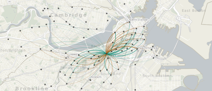 Credit:http://bostonography.com/hubwaymap/
This is a second part of Intra-National Migration data exploration. This post will also construt distance variables for the data and crack on with some Spatial Interction Modeling. This is a contribution to my PhD research that examines Origin-Destination and its spatial aspects.
Introduction
UK intra-migration data are open source data that can be downloaded from ONS. ONS uses the NHS Patient Register Data Service (PRDS) to find out the changes in patients adresses. Since most people change their address with their doctor soon after moving, these data are considered to provide a good proxy indicator of migration.
The migration data is published every year and consist of Origin Local Authority ID, Destination Local Authority ID, sex, age and movement factor field. This movement factor is based on resscaled number of people on the flow.
Please follow ONS to find more information about the methodology.
Follow Part 1 to see some basic graphs of the data.
Recap
I'm just going to quickly recap what we know alrady about the data.
- The origins and destinations are the same, UK Local Authorities.
- The flow volume is represented by movement factor wich is already scaled variable and is extremely skewed to the left.
- The year 2011 has very different nature from all the other years.
- Because we are not able to judstify the difference in nature of the 2011, we are going to work with the later years only.
In this post…
I want to calculate distances between the Originn and Destination.
Now, it might sound easy, but the theory behind this is more colmpicated than you would think. Read through my other post that explains most of the theory behind this.
I need to;
- Calculate the Eclidian Distance between the Origins and Destinations
- Calculate the Great Circle Distance between the Origins and Destinations
- Calculate the Network Distance (walking path along the streets)
1. Calculate the Euclidian Distance between the Origins and Destinations
To do that, we first need to load the libraries and the data we mungedin the post 1
# we will first import all necessary libraries
import pandas as pd
import os
import numpy as np
import glob
from datetime import datetime
import geopandas as gpd
import matplotlib.pyplot as plt
import seaborn as sns
import plotly.express as px
from shapely.geometry import Point, LineString
# set the path
file = r'./../data/migration/full_mig.csv'
# read the file
df = pd.read_csv(file, index_col=None, low_memory=False)
# plot the top of the table
df.head()
| OutLA | InLA | Age | Sex | Moves | Date | sex_bin | |
|---|---|---|---|---|---|---|---|
| 0 | E09000001 | E09000002 | 27 | 2 | 0.0002 | 2011-01-01 | 2 |
| 1 | E09000001 | E09000002 | 36 | 1 | 0.0004 | 2011-01-01 | 1 |
| 2 | E09000001 | E09000002 | 26 | 2 | 0.0004 | 2011-01-01 | 2 |
| 3 | E09000001 | E09000002 | 25 | 2 | 0.0005 | 2011-01-01 | 2 |
| 4 | E09000001 | E09000002 | 34 | 1 | 0.0014 | 2011-01-01 | 1 |
# set the path
file = r'./../data/migration/munged/LAcentrooids.shp'
# read the file in
la = gpd.read_file(file)
# show the map
la.plot();
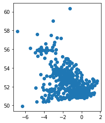
Now I can create lat and long columns in the centrooid data which I'll merge to the flow data twice. First based on the Out-flow LA ID and second based on In-flow LA ID.
# create new callumn x and y wit lat and long coordinates
la['x'] = la.geometry.x
la['y'] = la.geometry.y
la.head()
| objectid | lad17cd | lad17nm | geometry | x | y | |
|---|---|---|---|---|---|---|
| 0 | 1 | E06000001 | Hartlepool | POINT (-1.259479894328456 54.66947264221945) | -1.259480 | 54.669473 |
| 1 | 2 | E06000002 | Middlesbrough | POINT (-1.222265950359884 54.54199624640567) | -1.222266 | 54.541996 |
| 2 | 3 | E06000003 | Redcar and Cleveland | POINT (-1.020534867661266 54.55159000727666) | -1.020535 | 54.551590 |
| 3 | 4 | E06000004 | Stockton-on-Tees | POINT (-1.332307567288941 54.56157879321239) | -1.332308 | 54.561579 |
| 4 | 5 | E06000005 | Darlington | POINT (-1.552585765196361 54.54869927572448) | -1.552586 | 54.548699 |
# lets get rid of the rows we dont have spatial information for
# list of Unique ID's
d = list(la['lad17cd'].unique())
# new dataset with just those that are in a list
df2 = df.loc[df['OutLA'].isin(d)]
df3 = df2.loc[df2['InLA'].isin(d)]
# see how many rows we lost
len(df) - len(df3)
874611
# create two datasets from the la's base on Outflow and Inflow
# drop th geometries and create dataframes
outla = pd.DataFrame(la)
inla = pd.DataFrame(la)
# select just what we need
outla = outla.loc[:,['lad17cd','x','y']]
inla = inla.loc[:,['lad17cd','x','y']]
# rename the columns
outla.rename(columns = {'x':'out_x','y':'out_y'}, inplace = True)
inla.rename(columns = {'x':'in_x','y':'in_y'}, inplace = True)
# look at what we have
outla.head()
| lad17cd | out_x | out_y | |
|---|---|---|---|
| 0 | E06000001 | -1.259480 | 54.669473 |
| 1 | E06000002 | -1.222266 | 54.541996 |
| 2 | E06000003 | -1.020535 | 54.551590 |
| 3 | E06000004 | -1.332308 | 54.561579 |
| 4 | E06000005 | -1.552586 | 54.548699 |
# join the spatial points to the data, first for the OutLA and secondly for the InLA
df4 = df3.merge(outla, how = 'left', left_on = 'OutLA', right_on = 'lad17cd')
df4 = df4.merge(inla, how = 'left', left_on = 'InLA', right_on = 'lad17cd')
df4.tail()
| OutLA | InLA | Age | Sex | Moves | Date | sex_bin | lad17cd_x | out_x | out_y | lad17cd_y | in_x | in_y | |
|---|---|---|---|---|---|---|---|---|---|---|---|---|---|
| 10701098 | W06000024 | W06000023 | 67 | F | 1.1416 | 2018-01-01 | 2 | W06000024 | -3.361057 | 51.740942 | W06000023 | -3.409912 | 52.323737 |
| 10701099 | W06000024 | W06000023 | 73 | F | 0.9519 | 2018-01-01 | 2 | W06000024 | -3.361057 | 51.740942 | W06000023 | -3.409912 | 52.323737 |
| 10701100 | W06000024 | W06000023 | 74 | M | 1.0020 | 2018-01-01 | 1 | W06000024 | -3.361057 | 51.740942 | W06000023 | -3.409912 | 52.323737 |
| 10701101 | W06000024 | W06000023 | 74 | F | 0.9866 | 2018-01-01 | 2 | W06000024 | -3.361057 | 51.740942 | W06000023 | -3.409912 | 52.323737 |
| 10701102 | W06000024 | W06000023 | 77 | F | 3.0000 | 2018-01-01 | 2 | W06000024 | -3.361057 | 51.740942 | W06000023 | -3.409912 | 52.323737 |
# make sure there is no missing values
x = df4.isna()
x.loc[x['out_x'] == True]
| OutLA | InLA | Age | Sex | Moves | Date | sex_bin | lad17cd_x | out_x | out_y | lad17cd_y | in_x | in_y |
|---|
That looks like exactly what we need!
Next step will be calculating the Euclidian distance between the Drigin and the Destination.
There are actually quite few way to do this.
1. You can just use pythagoras function to do that
test = df4
test['Euc_distance'] = (((test.out_x - test.in_x) ** 2) + (test.out_y - test.in_y) ** 2) ** .5
test.head()
| OutLA | InLA | Age | Sex | Moves | Date | sex_bin | lad17cd_x | out_x | out_y | lad17cd_y | in_x | in_y | Euc_distance | |
|---|---|---|---|---|---|---|---|---|---|---|---|---|---|---|
| 0 | E09000001 | E09000002 | 27 | 2 | 0.0002 | 2011-01-01 | 2 | E09000001 | -0.092171 | 51.514845 | E09000002 | 0.133522 | 51.545272 | 0.227735 |
| 1 | E09000001 | E09000002 | 36 | 1 | 0.0004 | 2011-01-01 | 1 | E09000001 | -0.092171 | 51.514845 | E09000002 | 0.133522 | 51.545272 | 0.227735 |
| 2 | E09000001 | E09000002 | 26 | 2 | 0.0004 | 2011-01-01 | 2 | E09000001 | -0.092171 | 51.514845 | E09000002 | 0.133522 | 51.545272 | 0.227735 |
| 3 | E09000001 | E09000002 | 25 | 2 | 0.0005 | 2011-01-01 | 2 | E09000001 | -0.092171 | 51.514845 | E09000002 | 0.133522 | 51.545272 | 0.227735 |
| 4 | E09000001 | E09000002 | 34 | 1 | 0.0014 | 2011-01-01 | 1 | E09000001 | -0.092171 | 51.514845 | E09000002 | 0.133522 | 51.545272 | 0.227735 |
Very simple, we just need to pay attention to the units of the distance which is in degrees (coordinates of the points in degrees).
2. You can use scipy.spatial.distance.cdist() function that will basically do the same job, however needs more data manipulation
# import the library
# this could be done different ways too so feel free to do what suits you
import scipy.spatial.distance as ssd
# importing the library you use the the function as x=ssd.cdist()
from scipy.spatial import distance
# then use the function as x=distance.cdist()
import scipy
# then use the function as x=scipy.spatial.distance.cdist()
# Make selection
# I'll test this on selection of points as I did not find out why it does not like my vector of size 11575714...to big for this I guess
selection = test.iloc[0:5,:]
# to use this function, we neet to create numpy arrays from the coordinates, as the cdist() requires
coords_out = np.array(selection[['out_x','out_y']])
coords_in = np.array(selection[['in_x','in_y']])
# note that this function return a matrix
mat = distance.cdist(coords_out, coords_in, 'euclidean')
mat
array([[0.22773512, 0.22773512, 0.22773512, 0.22773512, 0.22773512],
       [0.22773512, 0.22773512, 0.22773512, 0.22773512, 0.22773512],
       [0.22773512, 0.22773512, 0.22773512, 0.22773512, 0.22773512],
       [0.22773512, 0.22773512, 0.22773512, 0.22773512, 0.22773512],
       [0.22773512, 0.22773512, 0.22773512, 0.22773512, 0.22773512]])
Then you need to convert the matrix into the collumn of the dataframe… I did not worked that one out, so let me know if you know how O:-)
However, BIG ADVANTAGE of this function is that it has predefined 24 different calculation of distances. Check out the documentation, and because it's based on C++ its quite fast.
2. Calculate the Great Circle Distance between the Origins and Destinations
This could be also done several ways.
The easiest way is using the GeoPy library, but if you find a faster way, let me know!
To do this we need to get the coordinates in one column as it was in original point dataset just stripped out of the geometry column.
from geopy.distance import geodesic, great_circle
import itertools
# create stripped column of coordinates
la['xy'] = la.geometry.apply(lambda x: [x.y, x.x])

# turn it into dataframe
points = pd.DataFrame(la)
# select just what we need
points1 = points.loc[:,['lad17cd','xy']]
points2 = points.loc[:,['lad17cd','xy']]
# rename the columns
points1.rename(columns = {'xy':'xy_1'}, inplace = True)
points2.rename(columns = {'xy':'xy_2'}, inplace = True)
# join the spatial points to the data, first for the OutLA and secondly for the InLA
test2 = test.merge(points1, how = 'left', left_on = 'OutLA', right_on = 'lad17cd')
test2 = test2.merge(points2, how = 'left', left_on = 'InLA', right_on = 'lad17cd')
test2.tail()
| OutLA | InLA | Age | Sex | Moves | Date | sex_bin | lad17cd_x | out_x | out_y | lad17cd_y | in_x | in_y | Euc_distance | lad17cd_x | xy_1 | lad17cd_y | xy_2 | |
|---|---|---|---|---|---|---|---|---|---|---|---|---|---|---|---|---|---|---|
| 10701098 | W06000024 | W06000023 | 67 | F | 1.1416 | 2018-01-01 | 2 | W06000024 | -3.361057 | 51.740942 | W06000023 | -3.409912 | 52.323737 | 0.584839 | W06000024 | [51.74094175880734, -3.361056696671829] | W06000023 | [52.323736681870706, -3.4099121042932894] |
| 10701099 | W06000024 | W06000023 | 73 | F | 0.9519 | 2018-01-01 | 2 | W06000024 | -3.361057 | 51.740942 | W06000023 | -3.409912 | 52.323737 | 0.584839 | W06000024 | [51.74094175880734, -3.361056696671829] | W06000023 | [52.323736681870706, -3.4099121042932894] |
| 10701100 | W06000024 | W06000023 | 74 | M | 1.0020 | 2018-01-01 | 1 | W06000024 | -3.361057 | 51.740942 | W06000023 | -3.409912 | 52.323737 | 0.584839 | W06000024 | [51.74094175880734, -3.361056696671829] | W06000023 | [52.323736681870706, -3.4099121042932894] |
| 10701101 | W06000024 | W06000023 | 74 | F | 0.9866 | 2018-01-01 | 2 | W06000024 | -3.361057 | 51.740942 | W06000023 | -3.409912 | 52.323737 | 0.584839 | W06000024 | [51.74094175880734, -3.361056696671829] | W06000023 | [52.323736681870706, -3.4099121042932894] |
| 10701102 | W06000024 | W06000023 | 77 | F | 3.0000 | 2018-01-01 | 2 | W06000024 | -3.361057 | 51.740942 | W06000023 | -3.409912 | 52.323737 | 0.584839 | W06000024 | [51.74094175880734, -3.361056696671829] | W06000023 | [52.323736681870706, -3.4099121042932894] |
# now calculate the great circle distance
# this takes good 15 min
test2['great_circle_dist'] = test2.apply(lambda x: great_circle(x.xy_1, x.xy_2).km, axis=1)
test2.head()
| OutLA | InLA | Age | Sex | Moves | Date | sex_bin | lad17cd_x | out_x | out_y | lad17cd_y | in_x | in_y | Euc_distance | lad17cd_x | xy_1 | lad17cd_y | xy_2 | great_circle_dist | |
|---|---|---|---|---|---|---|---|---|---|---|---|---|---|---|---|---|---|---|---|
| 0 | E09000001 | E09000002 | 27 | 2 | 0.0002 | 2011-01-01 | 2 | E09000001 | -0.092171 | 51.514845 | E09000002 | 0.133522 | 51.545272 | 0.227735 | E09000001 | [51.51484485100944, -0.09217115162643398] | E09000002 | [51.54527247765296, 0.13352209887032826] | 15.97471 |
| 1 | E09000001 | E09000002 | 36 | 1 | 0.0004 | 2011-01-01 | 1 | E09000001 | -0.092171 | 51.514845 | E09000002 | 0.133522 | 51.545272 | 0.227735 | E09000001 | [51.51484485100944, -0.09217115162643398] | E09000002 | [51.54527247765296, 0.13352209887032826] | 15.97471 |
| 2 | E09000001 | E09000002 | 26 | 2 | 0.0004 | 2011-01-01 | 2 | E09000001 | -0.092171 | 51.514845 | E09000002 | 0.133522 | 51.545272 | 0.227735 | E09000001 | [51.51484485100944, -0.09217115162643398] | E09000002 | [51.54527247765296, 0.13352209887032826] | 15.97471 |
| 3 | E09000001 | E09000002 | 25 | 2 | 0.0005 | 2011-01-01 | 2 | E09000001 | -0.092171 | 51.514845 | E09000002 | 0.133522 | 51.545272 | 0.227735 | E09000001 | [51.51484485100944, -0.09217115162643398] | E09000002 | [51.54527247765296, 0.13352209887032826] | 15.97471 |
| 4 | E09000001 | E09000002 | 34 | 1 | 0.0014 | 2011-01-01 | 1 | E09000001 | -0.092171 | 51.514845 | E09000002 | 0.133522 | 51.545272 | 0.227735 | E09000001 | [51.51484485100944, -0.09217115162643398] | E09000002 | [51.54527247765296, 0.13352209887032826] | 15.97471 |
YAAAAAAAAY
We have got a distance in kilometres!
Ok it's a mess, let's clean the dataset a little bit as there is several extra columns.
# create back up first
test3 = test2
test3 = test3[['OutLA','InLA','Age','Moves','Date','sex_bin', 'Euc_distance','great_circle_dist','out_x', 'out_y','in_x','in_y', 'xy_1','xy_2']]
test3.head()
| OutLA | InLA | Age | Moves | Date | sex_bin | Euc_distance | great_circle_dist | out_x | out_y | in_x | in_y | xy_1 | xy_2 | |
|---|---|---|---|---|---|---|---|---|---|---|---|---|---|---|
| 0 | E09000001 | E09000002 | 27 | 0.0002 | 2011-01-01 | 2 | 0.227735 | 15.97471 | -0.092171 | 51.514845 | 0.133522 | 51.545272 | [51.51484485100944, -0.09217115162643398] | [51.54527247765296, 0.13352209887032826] |
| 1 | E09000001 | E09000002 | 36 | 0.0004 | 2011-01-01 | 1 | 0.227735 | 15.97471 | -0.092171 | 51.514845 | 0.133522 | 51.545272 | [51.51484485100944, -0.09217115162643398] | [51.54527247765296, 0.13352209887032826] |
| 2 | E09000001 | E09000002 | 26 | 0.0004 | 2011-01-01 | 2 | 0.227735 | 15.97471 | -0.092171 | 51.514845 | 0.133522 | 51.545272 | [51.51484485100944, -0.09217115162643398] | [51.54527247765296, 0.13352209887032826] |
| 3 | E09000001 | E09000002 | 25 | 0.0005 | 2011-01-01 | 2 | 0.227735 | 15.97471 | -0.092171 | 51.514845 | 0.133522 | 51.545272 | [51.51484485100944, -0.09217115162643398] | [51.54527247765296, 0.13352209887032826] |
| 4 | E09000001 | E09000002 | 34 | 0.0014 | 2011-01-01 | 1 | 0.227735 | 15.97471 | -0.092171 | 51.514845 | 0.133522 | 51.545272 | [51.51484485100944, -0.09217115162643398] | [51.54527247765296, 0.13352209887032826] |
3. Calculating the network distances
I will demonstrate this on random points on Bristol as our migration data are not that relevant to a network distance. We just need to upload two libraries osmnx and networkx
There is nothing easier than get your network from osmnx, no need for looking for data and extra faf
import osmnx as ox
import networkx as nx
# define the place
place_name = "Bristol, United Kingdom"
# define the graph
graph = ox.graph_from_place(place_name, network_type='drive')
Now get some random points from Bristol
# 51.453700, -2.595778 # Dominos pizza in Bristol city centre
# 51.456294, -2.605236 # Bristol Gallery and Museum
# 51.468233, -2.588812 # Montpelier rail station
# 51.456569, -2.626453 # Clifton observatory

# create the list of coordinates
lat_list = [51.453700, 51.456294, 51.468233, 51.456569]
lon_list = [-2.595778, -2.605236, -2.588812, -2.626453]

#put it together
random_points = zip(lon_list, lat_list)

# create dataframe
random_points = pd.DataFrame(random_points)
# change the names of columns
random_points.rename(columns = {0:'x',1:'y'}, inplace = True)

# create spatial dataframe from the dataframe
random_points_gpd = gpd.GeoDataFrame(
    random_points, geometry=gpd.points_from_xy(random_points.x, random_points.y))
# assign coordinates
random_points_gpd.crs = la.crs
Now we need to convert everything to UTM as we want to get the lenght in metres not degrees
# define the crs
utm = "+proj=utm +zone=33 +ellps=WGS84 +datum=WGS84 +units=m +no_defs"
# points to utm
random_points_gpd = random_points_gpd.to_crs(utm)
# convert the graph into utm...projct_graph function does it all
graph = ox.project_graph(graph, to_crs = utm)
# lets just see how it looks like
fig, ax = ox.plot_graph(graph_proj)
plt.tight_layout()
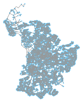
<Figure size 432x288 with 0 Axes>
# separate the nodes and edges from the graph
nodes_proj, edges_proj = ox.graph_to_gdfs(graph_proj, nodes=True, edges=True)
# look at the crs just to check
print("Coordinate system:", edges_proj.crs)
Coordinate system: +proj=utm +zone=33 +ellps=WGS84 +datum=WGS84 +units=m +no_defs
# create nearest nodes for each point

#get the coordinates only into dataframe
random_points_gpd['a'] = random_points_gpd.geometry.y
random_points_gpd['b'] = random_points_gpd.geometry.x
target_xy = pd.DataFrame(random_points_gpd[['a','b']])

# get the nearest node id for each row
def nearest_node(Lat,Lon):
    nearest_node,dist=ox.get_nearest_node(graph, (Lat,Lon), return_dist=True)
    return nearest_node

# apply the function
target_xy['node'] = np.vectorize(nearest_node)(target_xy['a'],target_xy['b'])
Now we create the Origin-Destination data this is going to be little fidly, indeed, but at least we have just a sample dataset
# separate just the node id
target2 = target_xy.iloc[:,[2]]

# double this for destinations
target3 = target_xy.iloc[:,[2]]
# reset the index and reverse the order
target3 = target3.sort_index(ascending=False).reset_index().reset_index()
target2 = target2.reset_index()

# merge those two node datasets into OD data
OD = target2.merge(target3, left_on='index', right_on= 'level_0')

# get rid of unnecessary columns
OD = OD.loc[:,['node_x','node_y']]
OD.head()
| node_x | node_y | |
|---|---|---|
| 0 | 6502760749 | 26127008 |
| 1 | 5432376184 | 358536159 |
| 2 | 358536159 | 5432376184 |
| 3 | 26127008 | 6502760749 |
# define a function that calculates shortest path between the nodes on graph
def short_path_length(row):
    return nx.shortest_path_length(graph, row['node_x'], row['node_y'], weight='length')

# apply the function to our OD data.....Note: as we are working with UTM projection, the units should be metres
OD['short_path_length'] = OD.apply(short_path_length, axis=1)
OD.head()
| node_x | node_y | short_path_length | |
|---|---|---|---|
| 0 | 6502760749 | 26127008 | 4537.728 |
| 1 | 5432376184 | 358536159 | 4031.132 |
| 2 | 358536159 | 5432376184 | 4039.488 |
| 3 | 26127008 | 6502760749 | 4611.492 |
Bare in mind I calculated the network distances on sample points in small area. That is because graph of whole UK is just huuuge and the computation would be time-expensive. In my opinion, we do not need the network distance for the migration data, however it could be usefull to know how to do that, so let me know if you found any quick and efficient way to do that.