Comparing the graph structures of the patients flow
# we will first import all necessary libraries
import pandas as pd
import os
import numpy as np
import glob
from datetime import datetime
import geopandas as gpd
import matplotlib.pyplot as plt
import seaborn as sns
import plotly.express as px
from shapely.geometry import Point, LineString
#from mpl_toolkits.basemap import Basemap
import osmnx as ox
import networkx as nx
import matplotlib as mpl
from networkx.algorithms import bipartite as bi
import statsmodels.api as sm
from scipy import stats
from statsmodels.formula.api import glm
wgs84 = {'init':'EPSG:4326'}
bng = {'init':'EPSG:27700'}
Prescription flow model validation
Using graphs to detect changes in spatial structure of the prescription flow
Using a graphs to look at the properties of the flow network, we need to first think about what kind of graph the network actually is and what kind of connections it has.
Based on the number of edges between two points we recognize
- Simple graph - Undirected graph with no loops and one edge between two points
- Multiple graph - Undirected graph with no loops
- Pseudograph - Graph with loops
Based on the type of the link we recognise;
- Undirected graph - the flow does not have a direction
- Directed graph - the flow have a direction, flow from point A to point B
We also recognize;
- Incomplete graph - graph in which at least one set of nodes is missing connection
- Complete graph - graph in which all the nodes are connected to all the other nodes
Lastly, we can also recognize very special case of a graph called Bipartite. What is Bipartiv graph? Recently, “bipartivity” has been proposed as an important topological characteristic of complex networks. A network (graph) G = (V,E) is called bipartite if its vertex set V can be partitioned into two subsets V1 and V2 such that all edges have one endpoint in V1 and the other in V2.
The GP and pharmacy flow are in nature Directed Incomplete pseudograph. that is because the flow goes from GP to pharmacy, always one direction, it does not contain the flows between all the pairs and also contains some loops; Gp can also dispense small amount odf prescriptions. Nevertheles, as the loops are very small proportoin of the data and we can benefit from the graph as a bipartite, I have attached dummy GPs into a pharmacy points so we can treat the loops as normal flows.
NOTE: what is the implication of this? We are loosing the information about connection of dome flows to origin, however, we are gaining an information on the process which reminds zero-inflated or hurdle process;
- Step 1 - patient come to GP but leaves without a prescriprion
- Step 2 - patient come to GP get the prescription virtually and recieve the drug from GP directly
- Step 3 - patient come to GP, get prescription, go to nearest pharmacy to get the drug
- Step 4 - patient come to GP, get the prescription and go to pharmacy close to shopping opportunity to get the drug
- Step 5 - patient come to GP, get the prescription and go to other pharmacy to get the drug
How do we represent the graph in Networkx?
Here are types of graphs in the networkx package
| Networkx Class | Type | Self-loops allowed | Parallel edges allowed |
|---|---|---|---|
| Graph | undirected | Yes | No |
| DiGraph | directed | Yes | No |
| MultiGraph | undirected | Yes | Yes |
| MultiDiGraph | directed | Yes | Yes |
We know our graph is directed so Digraph should serve the purpose. However, the data consist from monthly prescription flow so for most of the nodes we can find 12 edges throughout the year, so we need to work with MultiDiGraph to make sure we can account for all of those.
1. Load the data
# load the output of the gravity models, the flow data
# set the path
file = r'./../../data/NHS/working/predicted_flow_17.csv'
# read the file
flow17 = pd.read_csv(file, index_col=None)
# plot the top of the table
flow17.head()
| P_Code | P_Name_x | P_Postcode | D_Code_x | D_Name_x | D_Postcode | N_Items | N_EPSItems | Date | loop | ... | D_Left_y | D_X_y | D_Y_y | D_E_y | D_N_y | D_Setting_y | residents | Density | predict_items | predict_items_doubly | |
|---|---|---|---|---|---|---|---|---|---|---|---|---|---|---|---|---|---|---|---|---|---|
| 0 | L81004 | PORTISHEAD MEDICAL GROUP | BS20 6AQ | FA251 | HORIZON PHARMACY LTD | BS34 6AS | 130.0 | 0.0 | 2017-01-01 | False | ... | 20180115.0 | -2.562191 | 51.539195 | 361105.872423 | 182404.906640 | 50 | 456.517857 | 36.592857 | 29.316590 | 10.581379 |
| 1 | L81004 | PORTISHEAD MEDICAL GROUP | BS20 6AQ | FA613 | DOWNHAM FB LTD | BS7 9JT | 39.0 | 0.0 | 2017-01-01 | False | ... | NaN | -2.582219 | 51.480445 | 359664.895464 | 175881.865127 | 50 | 249.144737 | 54.493421 | 29.473430 | 2.853510 |
| 2 | L81004 | PORTISHEAD MEDICAL GROUP | BS20 6AQ | FCL91 | MYGLOBE LTD | BS15 4ND | 12.0 | 0.0 | 2017-01-01 | False | ... | NaN | -2.478870 | 51.459944 | 366826.940029 | 173549.785593 | 50 | 249.128205 | 30.569231 | 24.155556 | 2.061345 |
| 3 | L81004 | PORTISHEAD MEDICAL GROUP | BS20 6AQ | FCT35 | LLOYDS PHARMACY LTD | BS20 7QA | 661.0 | 0.0 | 2017-01-01 | False | ... | 20180131.0 | -2.758272 | 51.484474 | 347443.775309 | 176441.826480 | 50 | 369.081633 | 34.918367 | 1648.893267 | 1078.144522 |
| 4 | L81004 | PORTISHEAD MEDICAL GROUP | BS20 6AQ | FDD77 | JOHN WARE LIMITED | BS20 6LT | 4058.0 | 0.0 | 2017-01-01 | False | ... | NaN | -2.781349 | 51.481409 | 345837.744901 | 176117.839266 | 50 | 391.076923 | 29.092308 | 1194.123265 | 3570.014826 |
5 rows × 72 columns
# create a lists of the unique codes so we can subset the GP and PH point data
list_flow_GP = list(flow17['P_Code'].unique())
list_flow_PH = list(flow17['D_Code_new'].unique())
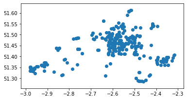
# get the pharmacies in
fl = './../../data/NHS/edispensary/PH_joined_daytimepop.geojson'
PH = gpd.read_file(fl)
PH = PH.to_crs(wgs84)
PH = PH[PH['D_Code_new'].isin(list_flow_PH)]
PH.plot();
C:\Users\tk18583\AppData\Local\Continuum\anaconda3\envs\geonet\lib\site-packages\pyproj\crs\crs.py:53: FutureWarning:

'+init=<authority>:<code>' syntax is deprecated. '<authority>:<code>' is the preferred initialization method. When making the change, be mindful of axis order changes: https://pyproj4.github.io/pyproj/stable/gotchas.html#axis-order-changes-in-proj-6
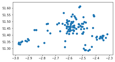
# get the GP's points in
GP = gpd.read_file("./../../data/NHS/epraccur/GP_AVON.geojson")
GP = GP[['P_Code','P_Name', 'full_address', 'P_Postcode', 'Open_date',
                                         'Close_date', 'Status_Code', 'Sub_type', 'Join', 'left', 'Setting', 'X', 'Y', 'geometry']]
GP = GP.rename(columns={'P_Postcode':'P_Postcode2','Open_date': 'P_Open_date', 'Close_date':'P_Close_date','full_address':'P_full_address' ,'Status_Code':'P_Status_Code', 'Sub_type':'P_Sub_type', 'Join':'P_Join', 'left':'P_Left', 'Setting':'P_Setting', 'X':'P_X', 'Y':'P_Y'}, errors="raise")
GP = GP.to_crs(wgs84)
GP = GP[GP['P_Code'].isin(list_flow_GP)]
GP.plot();
C:\Users\tk18583\AppData\Local\Continuum\anaconda3\envs\geonet\lib\site-packages\pyproj\crs\crs.py:53: FutureWarning:

'+init=<authority>:<code>' syntax is deprecated. '<authority>:<code>' is the preferred initialization method. When making the change, be mindful of axis order changes: https://pyproj4.github.io/pyproj/stable/gotchas.html#axis-order-changes-in-proj-6
2. Create a graph
We now know that the graph is bipartite, has multiple edges and has a directions, which means that we need to create MultiDiGraph. We also have weight on edge, that is the number of prescriptions on flow and predicted items on flow for both of the used models.
G1 = nx.from_pandas_edgelist(flow17, source='P_Code', target='D_Code_new', edge_attr=['N_Items'], create_using=nx.MultiDiGraph())
print('Is the graph bipirtite?   ' + str(nx.is_bipartite(G1)))
print('Is the graph directed??   ' + str(nx.is_directed(G1)))
Is the graph bipirtite?   True
Is the graph directed??   True
G2 = nx.from_pandas_edgelist(flow17, source='P_Code', target='D_Code_new', edge_attr=['predict_items'], create_using=nx.MultiDiGraph())
print('Is the graph bipirtite?   ' + str(nx.is_bipartite(G2)))
print('Is the graph directed??   ' + str(nx.is_directed(G2)))
Is the graph bipirtite?   True
Is the graph directed??   True
G3 = nx.from_pandas_edgelist(flow17, source='P_Code', target='D_Code_new', edge_attr=['predict_items_doubly'], create_using=nx.MultiDiGraph())
print('Is the graph bipirtite?   ' + str(nx.is_bipartite(G3)))
print('Is the graph directed??   ' + str(nx.is_directed(G3)))
Is the graph bipirtite?   True
Is the graph directed??   True
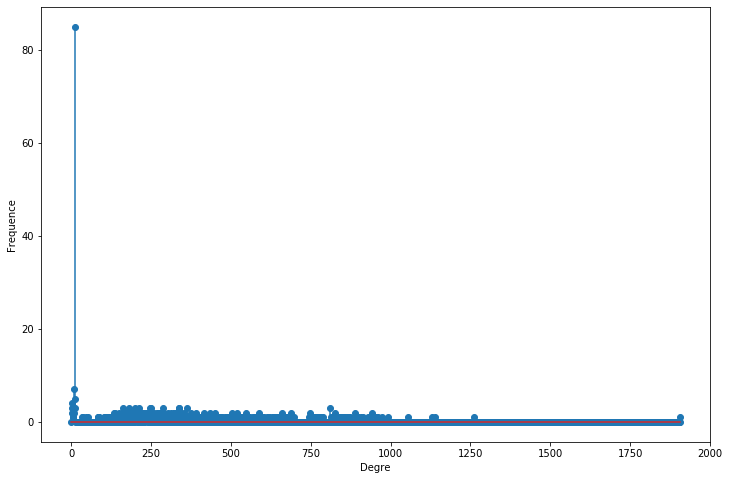
3. Look at the properties of the graph
# Look at number on graph properties
nb_nodes = len(G1.nodes())
nb_arr = len(G1.edges())
print("Number of nodes : " + str(nb_nodes))
print("Number of edges : " + str(nb_arr))
Number of nodes : 485
Number of edges : 74668
degree_freq = np.array(nx.degree_histogram(G1)).astype('float')
plt.figure(figsize=(12, 8))
plt.stem(degree_freq)
plt.ylabel("Frequence")
plt.xlabel("Degre")
plt.show();
C:\Users\tk18583\AppData\Local\Continuum\anaconda3\envs\geonet\lib\site-packages\ipykernel_launcher.py:3: UserWarning:

In Matplotlib 3.3 individual lines on a stem plot will be added as a LineCollection instead of individual lines. This significantly improves the performance of a stem plot. To remove this warning and switch to the new behaviour, set the "use_line_collection" keyword argument to True.
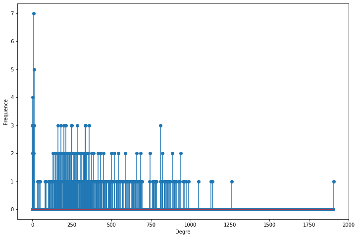
#degree_freq[degree_freq > 0]
x = degree_freq[degree_freq < 80]
plt.figure(figsize=(12, 8))
plt.stem(x)
plt.ylabel("Frequence")
plt.xlabel("Degre")
plt.show();
C:\Users\tk18583\AppData\Local\Continuum\anaconda3\envs\geonet\lib\site-packages\ipykernel_launcher.py:2: UserWarning:

In Matplotlib 3.3 individual lines on a stem plot will be added as a LineCollection instead of individual lines. This significantly improves the performance of a stem plot. To remove this warning and switch to the new behaviour, set the "use_line_collection" keyword argument to True.
plt.figure(figsize=(14,14))
nx.draw_networkx(G1, with_labels=True, width=0.02)
4. Define the functions to calculate centrality and snap the resluts to the point data
The Bipirtate graph is very specific cas of graph and has its own dedicated centraliy functions that can be calculated with networkx package.
This is the closeness and degree centrality, however none of those contain any weight, they are only based on the number of flows coming into the nodes.
No centrality can be measured in weighted bipirtite graph
Other measures we can look at are the Link Analysis measures. Those are Page Rank and HIIT (hubs and authorities). However, only Page Rank include a weight on edges,
Page Rank is the only measure we can apply on weighted directed bipartite graph!
def close_bi(graph, nodes, name, joinsA):
    # calculate the closenest
    close = bi.closeness_centrality(G = graph, nodes = nodes)
    # put it into a dataframe
    x = pd.DataFrame.from_dict(close,  orient='index')
    x = x.reset_index()
    x = x.rename({0: name},axis = 1)

    df = joinsA.merge(x, left_on = 'P_Code', right_on = 'index', how = 'left')
    return df

def degree_bi(graph, nodes, name, joinsA, joinsB):
    # calculate the closenest
    close = bi.degree_centrality(G = graph, nodes = nodes)
    # put it into a dataframe
    x = pd.DataFrame.from_dict(close,  orient='index')
    x = x.reset_index()
    x = x.rename({0: name},axis = 1)

    df = joinsA.merge(x, left_on = 'P_Code', right_on = 'index', how = 'left')
    df2 = joinsB.merge(x, left_on = 'D_Code_new', right_on = 'index', how = 'left')
    return df, df2

def pgr(graph, name, joinsA, joinsB, weight):
    # calculate the closenest
    close = nx.pagerank_scipy(G = graph, weight = weight, max_iter = 50)
    # put it into a dataframe
    x = pd.DataFrame.from_dict(close,  orient='index')
    x = x.reset_index()
    x = x.rename({0: name},axis = 1)

    df = joinsA.merge(x, left_on = 'P_Code', right_on = 'index', how = 'left')
    df2 = joinsB.merge(x, left_on = 'D_Code_new', right_on = 'index', how = 'left')
    return df, df2

# eigenvector centrality does not work for multidigraphs
def eigen_ce(graph, name, joinsA, joinsB, weight):
    # calculate the closenest
    close = nx.eigenvector_centrality(G = graph, max_iter = 100, weight = weight)
    # put it into a dataframe
    x = pd.DataFrame.from_dict(close,  orient='index')
    x = x.reset_index()
    x = x.rename({0: name},axis = 1)

    df = joinsA.merge(x, left_on = 'P_Code', right_on = 'index', how = 'left')
    df2 = joinsB.merge(x, left_on = 'D_Code_new', right_on = 'index', how = 'left')
    return df, df2
5. Apply the functions for Bipartate graph
GP2 = close_bi(graph = G1, nodes = list_flow_GP, name = 'close_G1', joinsA = GP)
GP2 = close_bi(graph = G2, nodes = list_flow_GP, name = 'close_G2', joinsA = GP2)
GP2 = close_bi(graph = G3, nodes = list_flow_GP, name = 'close_G3', joinsA = GP2)

GP2, PH2 = degree_bi(graph = G1, nodes = list_flow_GP, name = 'degree_G1', joinsA = GP2, joinsB = PH)
GP2, PH2 = degree_bi(graph = G2, nodes = list_flow_GP, name = 'degree_G2', joinsA = GP2, joinsB = PH2)
GP2, PH2 = degree_bi(graph = G3, nodes = list_flow_GP, name = 'degree_G3', joinsA = GP2, joinsB = PH2)

GP2, PH2 =  pgr(graph = G1, name = 'pgr_G1', weight = 'N_Items', joinsA = GP2, joinsB = PH2)
GP2, PH2 =  pgr(graph = G2, name = 'pgr_G2', weight = 'predict_items', joinsA = GP2, joinsB = PH2)
GP2, PH2 =  pgr(graph = G3, name = 'pgr_G3', weight = 'predict_items_doubly', joinsA = GP2, joinsB = PH2)

# eigenvector centrality does not work for multidigraphs
#GP2, PH2 =  eigen_ce(graph = G1, name = 'eig_G1', weight = 'N_Items', joinsA = GP2, joinsB = PH2)
#GP2, PH2 =  eigen_ce(graph = G2, name = 'eig_G2', weight = 'predict_items', joinsA = GP2, joinsB = PH2)
#GP2, PH2 =  eigen_ce(graph = G3, name = 'eig_G3', weight = 'predict_items_doubly', joinsA = GP2, joinsB = PH2)

GP2.drop(['index_x','index_y' ,'index'], axis=1, inplace=True)
PH2.drop(['index_x','index_y'], axis=1, inplace=True)
PH2.info()
<class 'geopandas.geodataframe.GeoDataFrame'>
Int64Index: 357 entries, 0 to 356
Data columns (total 25 columns):
 #   Column          Non-Null Count  Dtype
---  ------          --------------  -----
 0   D_Code          357 non-null    object
 1   D_Name          357 non-null    object
 2   D_full_address  357 non-null    object
 3   D_Postcode2     357 non-null    object
 4   D_Open_date     357 non-null    int64
 5   D_Close_date    27 non-null     float64
 6   D_Status_Code   357 non-null    object
 7   D_Sub_type      357 non-null    object
 8   D_Join          356 non-null    float64
 9   D_Left          27 non-null     float64
 10  D_X             357 non-null    float64
 11  D_Y             357 non-null    float64
 12  D_E             357 non-null    float64
 13  D_N             357 non-null    float64
 14  D_Setting       357 non-null    int64
 15  D_Code_new      357 non-null    object
 16  residents       357 non-null    float64
 17  Density         357 non-null    float64
 18  geometry        357 non-null    geometry
 19  degree_G1       357 non-null    float64
 20  degree_G2       357 non-null    float64
 21  degree_G3       357 non-null    float64
 22  pgr_G1          357 non-null    float64
 23  pgr_G2          357 non-null    float64
 24  pgr_G3          357 non-null    float64
dtypes: float64(15), geometry(1), int64(2), object(7)
memory usage: 72.5+ KB
# look at the values
GP2.iloc[:,14:23].head()
| close_G1 | close_G2 | close_G3 | degree_G1 | degree_G2 | degree_G3 | pgr_G1 | pgr_G2 | pgr_G3 | |
|---|---|---|---|---|---|---|---|---|---|
| 0 | 1.262397 | 1.262397 | 1.262397 | 1.456583 | 1.456583 | 1.456583 | 0.001684 | 0.001684 | 0.001684 |
| 1 | 1.262397 | 1.262397 | 1.262397 | 2.207283 | 2.207283 | 2.207283 | 0.001684 | 0.001684 | 0.001684 |
| 2 | 1.262397 | 1.262397 | 1.262397 | 1.834734 | 1.834734 | 1.834734 | 0.001684 | 0.001684 | 0.001684 |
| 3 | 1.262397 | 1.262397 | 1.262397 | 1.733894 | 1.733894 | 1.733894 | 0.001684 | 0.001684 | 0.001684 |
| 4 | 1.262397 | 1.262397 | 1.262397 | 0.806723 | 0.806723 | 0.806723 | 0.001684 | 0.001684 | 0.001684 |
PH2.iloc[:,19:25].head()
| degree_G1 | degree_G2 | degree_G3 | pgr_G1 | pgr_G2 | pgr_G3 | |
|---|---|---|---|---|---|---|
| 0 | 2.140625 | 2.140625 | 2.140625 | 0.002018 | 0.001812 | 0.001996 |
| 1 | 1.687500 | 1.687500 | 1.687500 | 0.002194 | 0.001957 | 0.002179 |
| 2 | 0.648438 | 0.648438 | 0.648438 | 0.001689 | 0.001774 | 0.001689 |
| 3 | 2.937500 | 2.937500 | 2.937500 | 0.002471 | 0.002330 | 0.002497 |
| 4 | 3.773438 | 3.773438 | 3.773438 | 0.001700 | 0.001867 | 0.001718 |
6. Changing graph structure
We can see that the degree centrality and closeness centraility is the same for all the graphs, because the wight is not included.
The Pagerank for the GP's is not changing either as the flows are leaving them and page rank focuses on the incoming flows only.
The Page Rank algorithm computes a ranking of the nodes in the graph G based on the structure of the incoming links, so we can only observe the importance of pharmacies.
plt.figure(figsize=(30, 6))
# Degree Centrality
f, axarr = plt.subplots(1,3, num=1)

plt.sca(axarr[0])
PH2['pgr_G1'].plot.hist(grid=True, bins=20, rwidth=0.9, color='#607c8e')
axarr[0].set_title('Page Rank Graph 1', size=16)

plt.sca(axarr[1])
PH2['pgr_G2'].plot.hist(grid=True, bins=20, rwidth=0.9, color='#607c8e')
axarr[1].set_title('Page Rank Graph 2', size=16)

plt.sca(axarr[2])
PH2['pgr_G3'].plot.hist(grid=True, bins=20, rwidth=0.9, color='#607c8e')
axarr[2].set_title('Page Rank Graph 3', size=16);
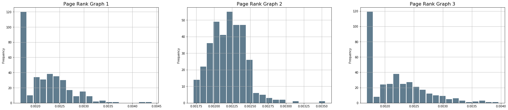
# which one is the most important? the one that sticks out
PH2[PH2['pgr_G1'] > 0.0044]
| D_Code | D_Name | D_full_address | D_Postcode2 | D_Open_date | D_Close_date | D_Status_Code | D_Sub_type | D_Join | D_Left | ... | D_Code_new | residents | Density | geometry | degree_G1 | degree_G2 | degree_G3 | pgr_G1 | pgr_G2 | pgr_G3 | |
|---|---|---|---|---|---|---|---|---|---|---|---|---|---|---|---|---|---|---|---|---|---|
| 112 | FLQ56 | BOOTS UK LIMITED | BOOTS UK LIMITED,59 BROADMEAD,BRISTOL,nan,BS1 3ED | BS1 3ED | 19480101 | NaN | A | 1 | 20040401.0 | NaN | ... | FLQ56 | 1021.5 | 202.028571 | POINT (-2.58972 51.45774) | 8.898438 | 8.898438 | 8.898438 | 0.004406 | 0.002691 | 0.003961 |
1 rows × 25 columns
ax = plt.figure(figsize=(10, 10))
plt.axis([PH2['pgr_G1'].min(), PH2['pgr_G1'].max(), PH2['pgr_G1'].min(), PH2['pgr_G1'].max()])
# plots
plt.scatter(PH2['pgr_G1'],PH2['pgr_G1'])
plt.scatter(PH2['pgr_G1'],PH2['pgr_G2'])
plt.plot(PH2['pgr_G1'].mean(),PH2['pgr_G1'].mean(), c = 'r', marker = 'X', markersize = 30)
# regression plots
sns.regplot(PH2['pgr_G1'],PH2['pgr_G1'])
sns.regplot(PH2['pgr_G1'],PH2['pgr_G2'])

plt.legend(['Mean','Page Rank from data', 'Page Rank from base gravity']);
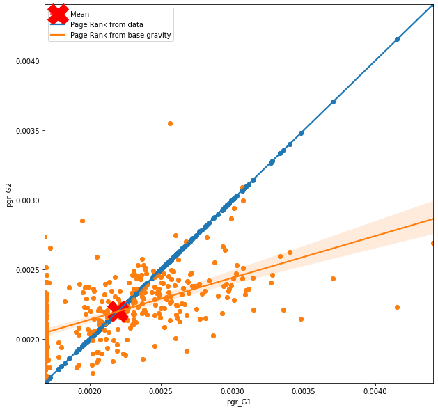
PH2['pgr_G1'].mean()
0.002197291434997281
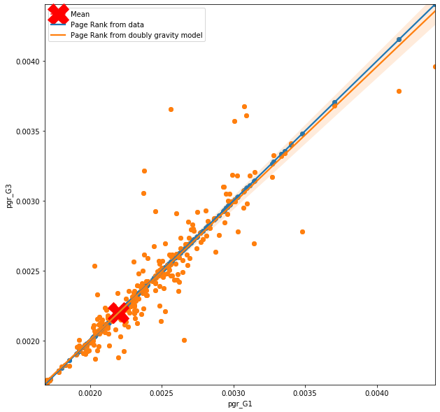
ax = plt.figure(figsize=(10, 10))
plt.axis([PH2['pgr_G1'].min(), PH2['pgr_G1'].max(), PH2['pgr_G1'].min(), PH2['pgr_G1'].max()])
# plots
plt.scatter(PH2['pgr_G1'],PH2['pgr_G1'])
plt.scatter(PH2['pgr_G1'],PH2['pgr_G3'])
plt.plot(PH2['pgr_G1'].mean(),PH2['pgr_G1'].mean(), c = 'r', marker = 'X', markersize = 30)
# regression plots
sns.regplot(PH2['pgr_G1'],PH2['pgr_G1'])
sns.regplot(PH2['pgr_G1'],PH2['pgr_G3'])

plt.legend(['Mean','Page Rank from data', 'Page Rank from doubly gravity model' ]);
Results
What we can see on the figure above is how the node centrality in the graph conctructed from prediction relates to a node centrality in the graph constructed from raw data. In ideal situation, the line of best fit and the observations would follow the blue line, however, this is not the case. From the first figure, which looks at the importance of the nodes based on base gravity model (very simple one), you can observe that where the actual importannce of the node is high, the importance based on predicted flows drop down drastically, and where the actual importance of the node is low, the importance based on predicted flows is higher. You can also notice line of zeros trying to hide behind the y axes. So although the model predicts flow with certain accuracy, th quality of the flow is not the same as from the data. More specifically the model is not really able to see the hierarchical structure of the nodes and creates predictions that are close to mean for all nodes.
Not suprisingly this is not the case for more complex gravity model such as doubly constrained gravity model. Here the hierarchy of the nodes is sustained by the prediction, however, that is expected as each node has it's own parameter in the model. Seems like a simple and smart solution, however, you need to remember the with doubly constrained model, where each node is considered as unique, predictions can be made only to existing nodes. So question like ‘What will happen with the flows if one of the GP's closes’ are hardly answerable. It's like a cheeky shortcut; if I am not able to meodel complicated flow structure, let's model each node separately.
Drop me a message on twitter if you have any comments :)