Introduction

If you have ever had anything to do with Origin-Destination (O-D) flow data and Spatial Interaction Models (SIM), you've probably wondered why there is so few application in a field, and why the Data Scientists are so hasitant with them. This article will help you to understand why is it so and where is the biggest problem.

If you know of some flow/O-D data and want to have your first try with a Spatial Interaction Models in R follow Dennett's Dr Ds Idiots Guide to Spatial Interaction Modelling for Dummies - Part 1: The Unconstrained (Total Constrained) Model and follow up with Dr Ds Idiots Guide to Spatial Interaction Modelling for Dummies - Part 2: Constrained Models. If you are a Python user, have a look into a SpInt package by Taylor Oshan, you can find working notebooks on GitHub. If you want to see how the SIMs are used see the Carto example.

I would say that there is one small problem and one big problem.

The small problem is most certainly the computational power. Unless you accessed a selection of the O-D data, the full datasets can be more than large. For example, the UK Intra-national migration data for one single year consist of between 1.5 to 2 milion records. If you look at 6 years of the migration data, you end up with 9 to 12 milion rows. For the flow data of population movement within a city on a daily bases, the longer period you're looking at the more data you have. Generally, most of the flow data or flow selections available are not that big in volume, so it should not be a problem for casual analyst with a casual computer. However, if you really bumb into a data that are so big that your computer can't deal with it, you should look into using your Graphics Processing Unit (GPU) to help you or ask for access to some High Performance Computer (HPC)

The big problem is the theoretical assumptions that underpin the methodology we use for the prediction. There you go, the rest of this post is all about the big methodology problem.

• I'll describe first the basic theory established back in a days and introduce a three major issues araising.
• Then, I'll follow up on each of those issues with alternative theories that has been introduced more recently.
• Finally, I'll sum it up into hopefuly short conclusion.

Background

You probably already know that the family of models we are talking about here are called Spatial Interaction Models (SIM's). SIM's capture the realitonship between two locations and are primarily based on gravity law. Gravity law is as old as sir Issac Newton and says that every particle attracts every other particle in the universe with a force which is directly proportional to the product of their masses and inversely proportional to the square of the distance between their center. In other words, all the origins and all the destinations are related to each other. The relationship between te origin and destination can be described by 3 information; firstly, the mass or any other variable that conceptually defines the size of the Origin, secondly, the mass or any other variable that conceptually defines the size of the Destination, and lastly, the distnce between Origin and Destiation. According to the Gravity law, this distance is mathematically defined as Inverse-square law, also called Power law, that could be very simply defined like this;

\begin{align} \alpha & = \frac{1}{distance^2} \end{align}

Te distance formula is the most important part of the interaction model, as it defines most of the relationshipp between the Origin and the Destination. It is also called a Distance-decay function and has been increasingly discussed in academia in the last half a century 1, 2, 3.

There are three fundamental problems with the Distancy-decay function.

1. The mathematical representation of the distance decay process.

2. The distance measure as itself.

3. The scaling issue

4. The unsuitability of the traditional distance measure for human cognitive environment.

This might at first sound confusing, so let me expain each point.

1. The problem with the math in distance decay function

Disclaimer first. Although I gone through university level math in my education, I'm no matematician! So do not expect any complicated formulas. I will try to describe the problems in a way that anyone can understand.

Already in early 20^th century, the scientists realized that the Inverse-square law, might not be the right function for the relationship they want to capture 4. Why is it so? Although it suggests some kind of scaling of the process, in high dimensions, it creates a ‘Dimensional Dilemma’. This mean that the ratio between the nearest and furthest points become uniformly distant from each other. Read this if you want to know more.

After the scientists reailized that this is just not going to work, another version of the distance-decay function has been introduced. The Inverse-square law was replaced with negative exponent. This is really simple;

\begin{align} distance^{-2} \end{align}

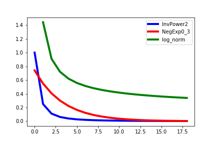
Negative exponent is much more suitable for the spatial interaction, because it does not suffer dimensionality issue, suggests locality and localization and descent little more intuitivly to the real descent observed in the data. You can see how this looks like on a graph below.

You can try this by yourself! Try this little simulation in R;

library(reshape2)
library(ggplot2)

xdistance <- seq(1,20,by=1)
InvPower2 <- xdistance^-2
NegExp0.3 <- exp(-0.3*xdistance)
log_norm <- 1/log(xdistance)
df <- cbind(InvPower2,NegExp0.3, log_norm)
meltdf <- melt(df)
ggplot(meltdf,aes(Var1,value, colour = Var2)) + geom_line()

OR in Python

import numpy as np 
import pandas as pd
import matplotlib.pyplot as plt

xdistance = np.arange(1, 20, 1, dtype='float32')
InvPower2 = 1/xdistance ** 2
NegExp0_3 = np.exp(((-0.3)*xdistance))
log_norm = 1/np.log(xdistance)
df = pd.DataFrame({'InvPower2':InvPower2, 'NegExp0_3':NegExp0_3, 'log_norm':log_norm})
plt.plot('InvPower2' , data = df, color='blue', linewidth=4)
plt.plot('NegExp0_3' , data = df, color='red', linewidth=4)
plt.plot('log_norm' , data = df, color='green', linewidth=4)
plt.legend();

BUT the negative exponent actually violets everything we know about spatial interaction, it viloates the first law of Geography by W. Tobler5. Although it suggests locality, it simply cannot reflect the interaction between two distant places.

Furthermore, recent paper from Broido & Clauset(2019) proves that for most of the natural flow networks, log-normal function fits the distribution better than or at least as well as Power of law. You can see it's shape on Figure 1 and formula as follows;

\begin{align} \alpha & = \frac{1}{log(distance)} \end{align}

Different transformation have different positives and negatives. See Taylor, 1971 for an overview on transformation functions in distance-decay function. But one thing is clear, none of them is the one transformation applied for all. Yes, as same as in the Lord of the Rings, transformation functions fight together agints the old rule (Power law) and want to achieve independence for each case.

It is undeniable that each case of flow network with its own scale, variability and character will assign different value to a distance. This result in neverending hunt for the right distance decay function. In fact, with a recent progresses in the society such as better transport networks, better mobility, better accessibility and of course presence of internet and social media, some suggest that the effect of distance on flow networks deminishes, especially in developed countries.

2. The distance measure as itself.

Other than the fact that the distance decay function remains arguable, the scientists also discuss what measure they could use for the distance. In traditional spatial interaction models this is a straight distance from origin to destination, which in many cases means Euclidean distance. Euclidian distance ranges from 0 to 1 and is usually used in virtual networks.

You can already feel that voice in your head that goes “This is very fishy, most of the networks are not virtual!". Absolutely! most of the flow networks you can find wil probably be constrained to earth space, where we masure distance by metric system. Sraight distance on earth is represented by Great Circle distance in metres, kilometres and other units we use.

Oh, here is the voice in your head again! You can already tell that this might be suitable for a airplane or ship networks because those actually move on the straight line on earth or maybe some organisms like bacteria as well. But when it comes to humans, human actions or animals, the movement more often follows some kind of predifined network that creates constraints to our movement. This could be pathways, roads, river banks or other. We called this Network distance.

And there is more. Some flow networks require an alternative measure of the distance. for example for subway or other public transport flow networks, travel time seem to be more representative to human behaviour on the network. One of the most groundbraking ways to suplement a distance measure could be a recent developement of the Radiation models. Those uses population in radiation distance between origin and destination as an indication of flow probability. You can read the initial paper here.

Again, the choice of distance measure is dependent on each individual case of network, so the hunt continues.

3. The Scaling issue

Everything in the Geography and Social Sciences is subject to scale. Whole multilevel modelling field was based on the fact that phenomena observed on individual level might not be relevant to wider or global population. And that is also a case for the SIMs.

We might have not noticed at first as most of the accessible interaction data are fixed for certain level. Notice that most of the flow data has a clear definition of location in the name or any other condition that constraints the amount of flow or the nature of them; inter-city migration, intra-national migration, inter-national migration, commuters flow, national-park visitors flow, shoppers flow, railway network, cycle path network. But, when you think about it, these are nothing else than selections of the actual data that restrict the data variability.

The only reason why we actually sticked to those one level interactions is because there is less data (no need for special hardware or software), but mainly because they nature of the data follows more or less a same idea. If the flows has all same nature, they will more likely fit the same mathematic rule and allows us the use some of the simplified models we talked about previously, such as gravity model with negative exponent distance-decay. You simply cannot apply the same function for interaction of few individuals and interaction of masses.

This issue of scale has been increasingly discussed in past two decades 5, 6. One of the major realization we made is that although we restrict the data, the scaling issue is still present. This is because there is many ways to define a scale in interaction. It could be the distance traveled, the purpose of the flow, the transport type and even the individuals demographics. As an example take the London commuter flows. The commuters can use any type of transport, they can commute from anywhere in London but also as far as from other parts of the country, they commute daily or weekly and can commute to school, work or for other purposes. In other words, Spatial interaction is subject of multiple scaling issues that are usually not related; we don't expect all the man commuting to work or all the commuters to use tube. Bulding a model for such a complex problem is not suprisingly almost impossible with the traditional methodology.

Luckily, there has been lately an interest in this issue and scientists are attempting to build an universal models of mobility. Those are leaning towards two fairly diverse approaches. Application of Machine Learning 7 and implementation of Game Theory 8. Those seem to be very promissing, however, more robust evidence is needed for validating both of these aproaches for various flow networks.

4. The unsuitability of the traditional distance measure for human cognitive environment.

The last but not least, there is the nature of the flow that determines what kind of distance is the most suitable for the model. But what is the nature of the flow?

Human flows especially can be very complex in the nature. They individuals flow is dependent on the individuals experience, character, gender, age, perception, socio-economic status and all the other attributes that shape our decisison making process. Already Hanson, 1981 claims that individual patterns are not of constant variability, both in space time and that they are far more complex than it is recognized in simple measures, such as frequency of trips and its distance.

The only common pattern in this mess could be the constrains form our society that apply to all of us. For example, most of us go to work or school, most of us has families, most of us uses weekend for leisure activities and most of us do not want to trade to much of our time for excessive travelling, and so minimize our space-time utility. For vast majority of the society same economic rules apply, hence it is probably incorrect to assume that choice actually exists for other than very few groups of people, differentiated on the basis of the socio-economic status. Not enough research has been conducted on the certainty and uncertainty of human movement patterns.

If you are more interested in this, I would recomend a book “Spatial Behaviour” from R. Golledge.

Conclusion

The distance-decay function has been the most variable and unstable subject of scientific interest in past few decades. That does not necessarily mean that there is no availiable solution for this issue.

The most promissing approach to spatial interaction are Spatial Autoregressive (SAR) models developed by L. Anselin, 1988. Intoduction of spatial effects in form of spatial weights to Interaction models supports the First Law of Geography and proved to be very efficient in predicting flows. Yet some limitations still exist and the question that has not been answered yet is about the degree randomnes of human behaviour patterns.

Well, now you know that spatial interaction models can be more complex than it seems from the outside. I hope you understand why are data scientist so hasitant with their application and if you ever have a project of such kind, be carefull with your models specifications and justification of the theoretical assumpions.