Czech trains, usage across the country
In past two years, Czech people experienced significant changes in the Czech Railway system. Here, I’m looking into the data published by XX to see what was the effect of those changes on the railway network usage.
Introduction
Public transport in Czech Republic has always been reliable and the most convenient transport thanks to it’s wide network reaching almost every conner of the country. From the previous government regime, people also got used to very low prices, that allowed everybody to use trains on everyday basis, However, this might have been also a way of the past government to regulate the car ownership amongst the population and so regulate the population movement out of the country.
Since the Czech Rebupblic gained independency, the railway system did not change drastically. It was run by a Czech National Railway monopol until the late 2000’s, when new privaty company ‘Regiojet’ was introduced to the public. The Regiojet has revolutionized the standards of the train service, but also the job market and the railway standards. Their trains had better service, more comfortable seating and cheap food on board. This made Czech population to prefer a private company over the National Railways. In this time, prices were higher due to inflation but remained farly low, allowing the students and seniors claim 25-30% discount on tickets.
Due to a constant and repetitive complaints from the young and elder population, the government made a decision in 2018 to increase the discount for students and seniors to 75%. This has been welcomed part of the population and has been succesfull for fist half a year. However, with such a drastic change, the railway companies started to loosing funds and annonced that if the ticket prices going to remain same, the railway system will collapse.
In February 2019 the Czech National Railwas also introduced a Flexi rates. On the example from the western countries, the ticket prices are flexible, depending on the day of the purchase (the earlier the cheaper), the time of the day the the train goes (peak, off-peak) and the freqency of the route (more frequented routes such as Prague-Ostrava are more expensive).
Keep in mind that the average hourly wage in Czech Republic is between 3-4 pounds which makes you work one whole day for one ticket.The wages obviously differ by job position, but they also differ signifficantly by region. For example, part time waitress in Prague can get up to 5 pounds an hour without tips, in compare with 3 pound an hour for same position in the Ostrava city.
Motivation
While spending the Christmas at my Czech home, I witnessed the effect of the changes by my own wallet. Therefore, I decided to investigate the changes in the usage of the railway network by analysing avaliable open source data. This is also a learning tutorial for those who work with R.
Data
The data on number of travelers on Czech trains arriving to each regions were retrieved from the 2018 Yearly Report of Czech National Trains.
Data on the number of travelers on Czech trains traveling within regions were retrieved from the same report. However, needed to be manually put together, as the reports provide separate table for each region.
Structure of the Czech regions and railway network
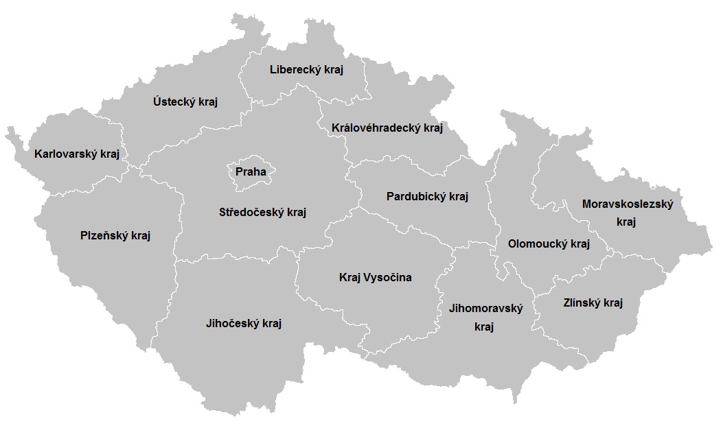
Figure 1: Czech regions (https://commons.wikimedia.org/wiki/File:Samospr%C3%A1vn%C3%A9_kraje.png)
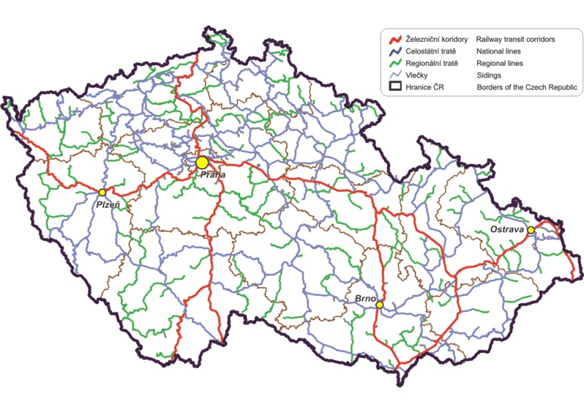
Figure 2: Railway network structure (https://www.sydos.cz/cs/rocenka-2005/rocenka/htm_cz/cz05_902000.html)
library(rgdal)
library(readxl)
library(reshape2)
library(ggplot2)
library(ggridges)
library(ggpubr)
# Read the data into a table
vl = read_xls('data/cz18_530112.xls')
vl # show the top of the table## # A tibble: 15 x 7
## area `2010` `2014` `2015` `2016` `2017` `2018`
## <chr> <dbl> <dbl> <dbl> <dbl> <dbl> <chr>
## 1 Stredoceský kraj 5787 13233 13973. 14044. 14346. 15041.142
## 2 Jihoceský kraj 393 419 461. 520. 758. 764.0299999999~
## 3 Plzenský kraj 319 429 498. 553. 658. 713.8400000000~
## 4 Karlovarský kraj 80 99 112. 122. 189. 148.8499999999~
## 5 Ústecký kraj 1089 793 806. 950. 902. 941.1900000000~
## 6 Liberecký kraj 67 67 66.7 70.5 84.8 83.29000000000~
## 7 Královéhradecký k~ 272 374 376. 386. 486. 548.3200000000~
## 8 Pardubický kraj 724 905 984. 1030. 1319. 1247.813000000~
## 9 Kraj Vysocina 198 210 210. 217. 261. 277.1499999999~
## 10 Jihomoravský kraj 237 458 543. 655. 1081. 1131.766000000~
## 11 Olomoucký kraj 423 843. 978. 1088. 1442. 1198.258
## 12 Zlínský kraj 178 227. 256. 288. 415. 357.154
## 13 Moravskoslezský k~ 452 924. 1036. 1117. 1577. 1204.643
## 14 Celkem príjezdy 10219 18980. 20299. 21041. 23518. 23657.446
## 15 <NA> NA NA NA NA NA Zdroj: MDWe can see that the table is organized as a wide table it has the region names as first collumn and the every other collumn specify the year in which certain number of people travaled. We can also notice that there is 15 rows, however the the 15th is empty and the 14th represent totals for a year.
If we want to analyze the data, we need to;
- Delete rows that does not need to be there
- Reshape the data from wide to long
- Transform the variables into usable ones
# create new table with only first 13 rows of the original table and keep the original
vl1 = vl[1:13,]
vl1$`2018` = as.numeric(vl1$`2018`)

# reshape the data from wide to long
vl1 = melt(data = vl1, id.vars='area', variable.name = 'year', value.name = 'Noftravelers' )
# id.vars represent the unique identification for the regions, which we want to keep in first collumn
# variable.name represent variable that will be created from al the other collumn names
# value.name represents the name of the column with will hold the cell values, here the number of travelers

# transform the value variable into numeric type, so we can use it as a number
vl1$Noftravelers = as.numeric(vl1$Noftravelers)
# transform the year into date type variable, so we can use a time-series
vl1$year = as.Date(vl1$year, '%Y')
# transform the regions name into factors
vl1$area = as.factor(vl1$area)
# change the names of the regions for simple text without interpunction, R doesn't like it
levels(vl1$area) <-  c("Jihocesky kraj", "Jihomoravsky kraj", "Karlovarsky kraj", "Kraj Vysocina", "Kralovehradecky kraj","Liberecky kraj","Moravskoslezsky kraj", "Olomoucky kraj", "Pardubicky kraj", "Plzensky kraj", "Stredocesky kraj" , "Ustecky kraj", "Zlinsky kraj")
Now when we cleaned the data, we can have a look at some basic time-series.
# use ggplot the create plot with lines (geom_line), for each region in time
a = ggplot(vl1, aes(x=year, y=Noftravelers, colour = area)) + ggplot2::geom_line()
a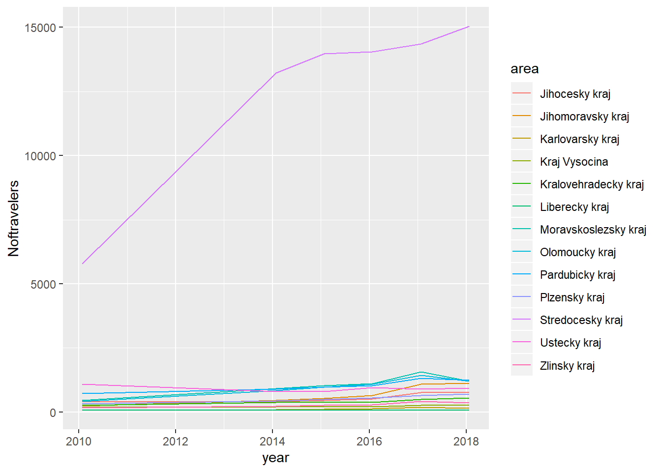
This plot shows that the Stredocesky kraj (Middle Bohemian region that includes Prague) has the highest flow of the travelers through the time. Moreover, their number continuously increases. We could suspect that that is a result of attractive job opportunities in the Capital Prague.
Note that the as.Date function creates complete date record that supply today’s date into the missing fields. This means that our dates are all fixed to 27th December. The results of this is litte confusing plot which actually shows the 2015 record at the break just before 2016
Let’s have a look at the rest of the regions only and compare the two plots and make it a bit prettier; add axes labels and title.
# build up the second plot
b = ggplot(vl1[vl1$area != "Stredocesky kraj",], aes(x=year, y=Noftravelers, colour = area)) + ggplot2::geom_line() + ggtitle("Train usage in Czech Republic by regions") + xlab("Year") + ylab("Number of travelers (in thousands)")

b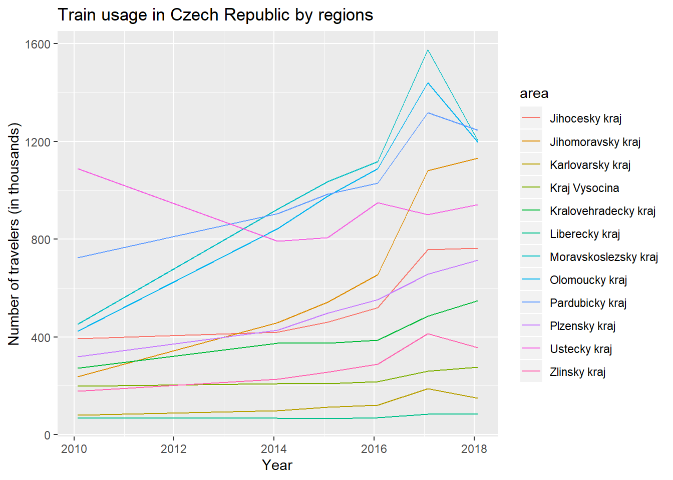
We can see that the number of passangers travelling into the regions is still continously increasing for most of the regions except Ustecky kraj, which decreases at first. We can also notice very visible peak on 2017, similar for all of the regions, which drops down significantly in 2018.
Overall, we could conlcude that some changes in travelers behaviour are definitely happenning, at least if it comes to travelers arriving to regions. Specifically, there is a visible increase in 2017 and decrease in 2018, which is the stronger in some regions of Czech Republic
What else?
We can also have a look on the number of travelers that travel within the same region to see if we can spot some anomalies as well.
# Read the data into a table
wr = read_xls('data/withinCZ.xls')
Now clean the data the same way as the previous.
# fix the fields to make sure the number converts corectly
wr$`2010` = as.numeric(wr$`2010`)
wr$`2014` = as.numeric(wr$`2014`)
wr$`2015` = as.numeric(wr$`2015`)
wr$`2016` = as.numeric(wr$`2016`)
wr$`2017` = as.numeric(wr$`2017`)
wr$`2018` = as.numeric(wr$`2018`)

wr1 = melt(data = wr, id.vars='area', variable.name = 'year', value.name = 'Noftravelers' )
wr1$Noftravelers = as.numeric(wr1$Noftravelers)
wr1$year = as.Date(wr1$year, '%Y')
wr1$area = as.factor(wr1$area)
ggplot(wr1, aes(x=year, y=Noftravelers, colour = area)) + ggplot2::geom_line() + ggtitle("Train usage within the same region") + xlab("Year") + ylab("Number of travelers (in thousands)")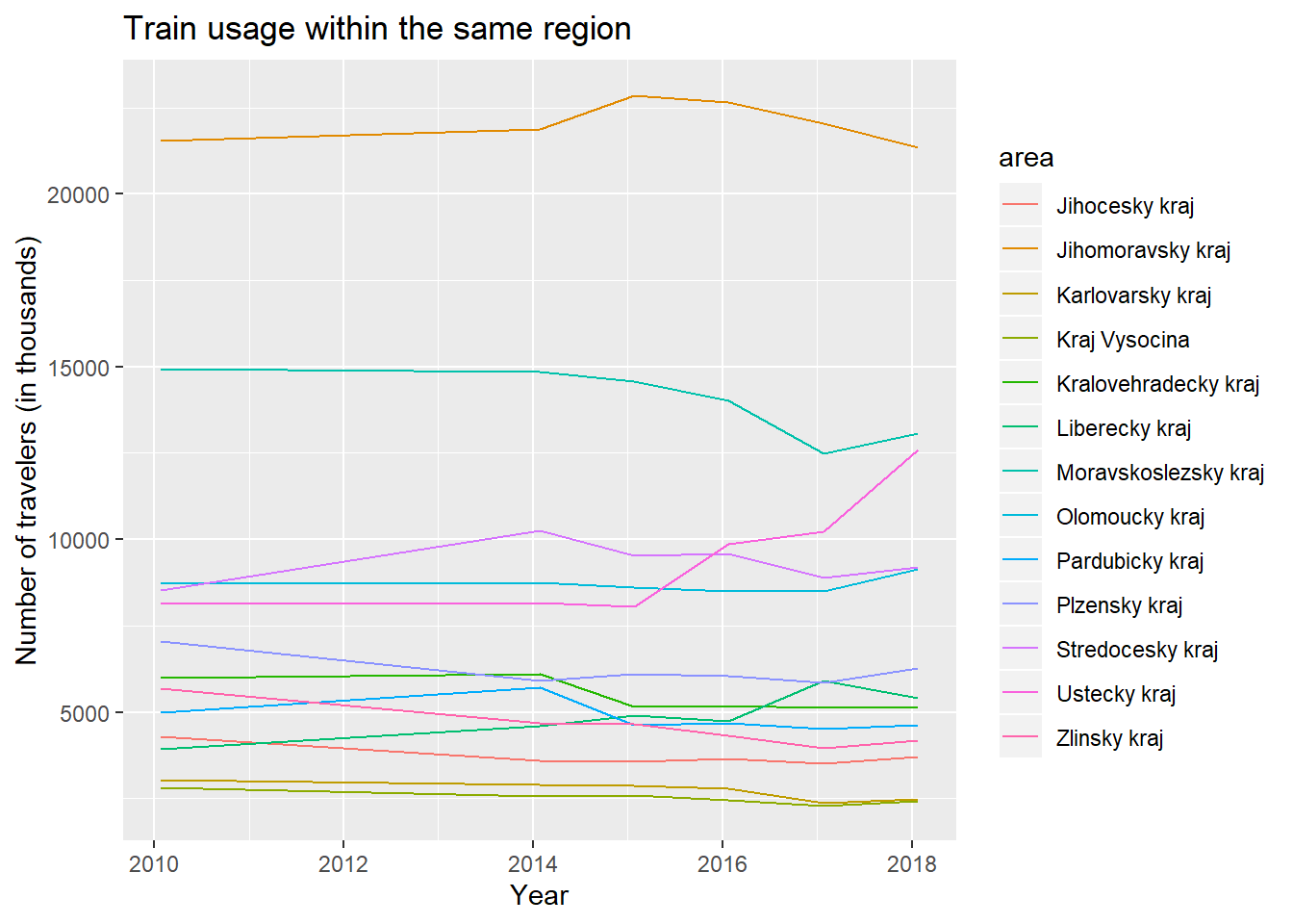
It looks like there is a less fluctation on train usage within the regions. The highest number of traveres use trains within the Jihomoravsky kraj and the Moravskoslezsky kraj just below. Those regions are the ones furthest away from the capital (Figures 1 and 2). There is some fluctation between 2015 and 2018. In some regions the intraregional travelers slightly increase and some decrease. However, we cannot recognize any clear trend.
Conclusion
Since the introduction of 75% discount and the flexi train tickets in Czech railway system, we can notice some changes of travelers behavior. People changed their train journey preferences, which caused unexpected fluctation in train usage. However, those changes are clearly visible only on train usage between the regions, while the changes of train usage within the regions remain unclear.
We must note that these graphs are only as good as the data. And because the workflow of how these data are generated is not known, please refer to Transport statistic by the Czech Ministry of Transport to see more information.
Let me know your thoughts, happy coding!
# Information about dependencies and the R version
# Keep in mind that some of the packages are not needed in the analysis and servers to the website creation process; blogdown, yaml, ...
sessionInfo()
## R version 3.6.1 (2019-07-05)
## Platform: x86_64-w64-mingw32/x64 (64-bit)
## Running under: Windows 10 x64 (build 18362)
##
## Matrix products: default
##
## locale:
## [1] LC_COLLATE=English_United Kingdom.1252
## [2] LC_CTYPE=English_United Kingdom.1252
## [3] LC_MONETARY=English_United Kingdom.1252
## [4] LC_NUMERIC=C
## [5] LC_TIME=English_United Kingdom.1252
##
## attached base packages:
## [1] stats graphics grDevices utils datasets methods base
##
## other attached packages:
## [1] ggpubr_0.2.4 magrittr_1.5 ggridges_0.5.1 ggplot2_3.2.1
## [5] reshape2_1.4.3 readxl_1.3.1 rgdal_1.4-6 sp_1.3-1
##
## loaded via a namespace (and not attached):
## [1] Rcpp_1.0.2 cellranger_1.1.0 compiler_3.6.1 pillar_1.4.2
## [5] plyr_1.8.4 tools_3.6.1 zeallot_0.1.0 digest_0.6.21
## [9] evaluate_0.14 tibble_2.1.3 gtable_0.3.0 lattice_0.20-38
## [13] pkgconfig_2.0.3 rlang_0.4.1 cli_1.1.0 yaml_2.2.0
## [17] blogdown_0.17 xfun_0.10 withr_2.1.2 stringr_1.4.0
## [21] dplyr_0.8.3 knitr_1.25 vctrs_0.2.0 grid_3.6.1
## [25] tidyselect_0.2.5 glue_1.3.1 R6_2.4.0 fansi_0.4.0
## [29] rmarkdown_1.16 bookdown_0.16 purrr_0.3.3 backports_1.1.5
## [33] scales_1.0.0 htmltools_0.4.0 assertthat_0.2.1 colorspace_1.4-1
## [37] ggsignif_0.6.0 labeling_0.3 utf8_1.1.4 stringi_1.4.3
## [41] lazyeval_0.2.2 munsell_0.5.0 crayon_1.3.4